Wave-based liquid-interface metamaterials

Abstract

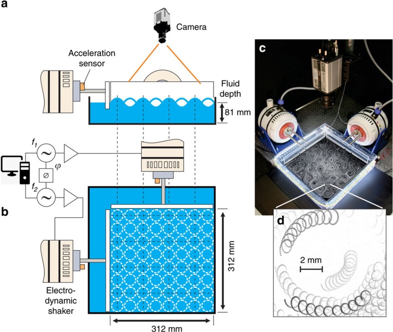
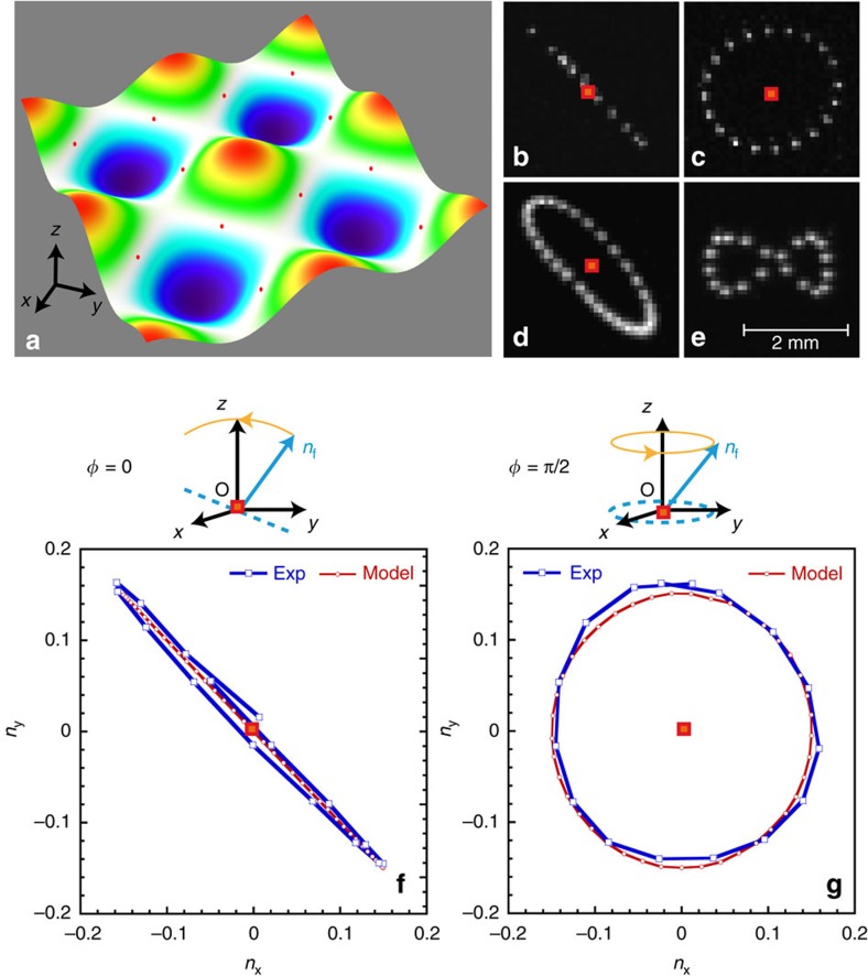
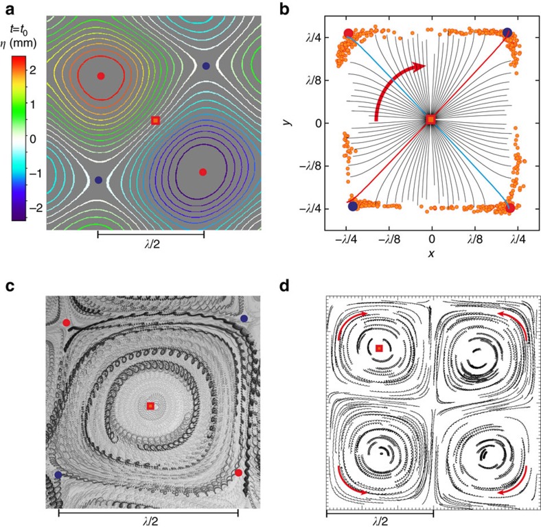
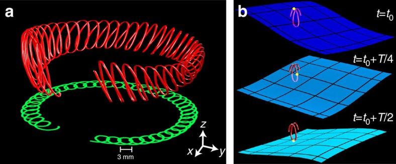
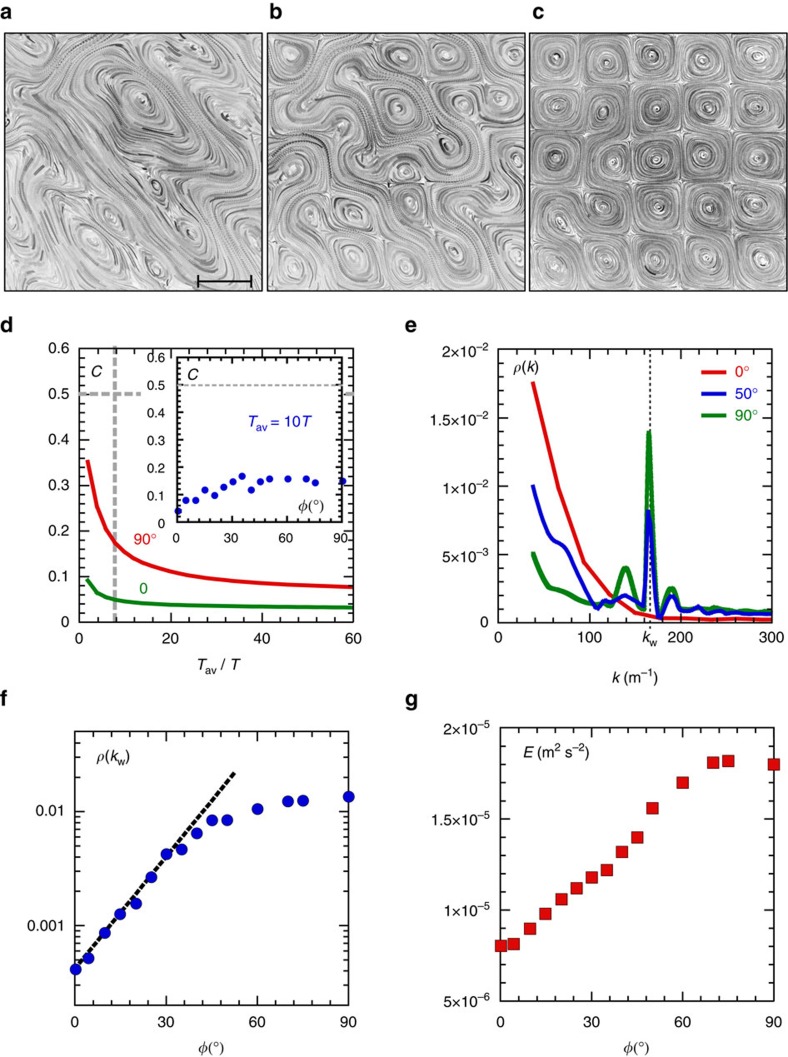
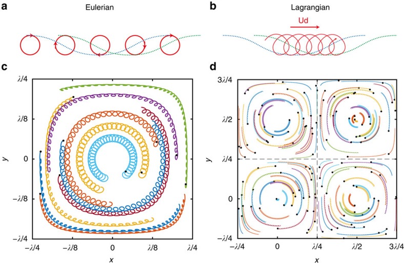
The control of matter motion at liquid-gas interfaces opens an opportunity to create two-dimensional materials with remotely tunable properties. In analogy with optical lattices used in ultra-cold atom physics, such materials can be created by a wave field capable of dynamically guiding matter into periodic spatial structures. Here we show experimentally that such structures can be realized at the macroscopic scale on a liquid surface by using rotating waves. The wave angular momentum is transferred to floating micro-particles, guiding them along closed trajectories. These orbits form stable spatially periodic patterns, the unit cells of a two-dimensional wave-based material. Such dynamic patterns, a mirror image of the concept of metamaterials, are scalable and biocompatible. They can be used in assembly applications, conversion of wave energy into mean two-dimensional flows and for organising motion of active swimmers.

Figure 1. Experimental set-up.

(a,b) Schematics of the experimental set-up for the controlled superposition of two orthogonal standing waves in a fluid tank. Waves are created using two computer controlled electrodynamic shakers. The amplitudes, frequencies and relative phase of the two waves are adjusted with high accuracy. Both the wave field and the surface flow can be measured (see ‘Methods' section for details). (c) A photo of the laboratory set-up showing the time-averaged streaks of drifting imaging particles. (d) Zoom into spatially resolved, small-scale particle drifting orbits.

Figure 2. Surface elevation and surface particle orbits near the nodal points.

(a) Measured surface elevation produced by two orthogonal standing waves. Red dots indicate positions of nodal points. (b–d) Orbits of the surface particles near the nodal points (red squares) for different phase shifts φ between the standing waves: (b) φ=0, (c) φ=π/2 and (d) φ=π/4. The orbital motion is measured over one wave period T=2π/ω≈0.26 s. (e) A particle orbit near a nodal point for ω₁=2ω₂. (f,g) Temporal trace (over T) of the horizontal projections (n_x, n_y) of the water surface normals (n_f in the schematics) at a nodal point for f φ=0 and g φ=π/2. Experimental measurements are compared with the theoretical model (see ‘Methods' section) for ω₁=ω₂, f=ω/2π=3.9 Hz (λ=104 mm) and H=1 mm.

Figure 3. Surface topography and fluid particle trajectories at the surface for φ=π/2.

(a) Contour plot of the surface elevation η measured at the half-wavelength scale and t=t₀. The positions of a nodal point (red square), peaks/troughs (red circles) and saddle points (blue circles) are highlighted. (b) Dynamics of the rotating wave about a nodal point within a unit cell of size L_c=λ/2. Orange circles: motion of wave peaks experimentally tracked for 50T. Black lines: the rotation of the z=0 isoline of the surface elevation followed for T/2. (The red line indicates t=t₀, the blue one t=t₀+T/4.) (c,d) Surface particle drifts tracked for ≈50T: (c) within a single unit cell, particle orbits drift forming closed nested guiding centre trajectories (experiments, f=ω/2π=3.9 Hz (λ=104 mm), H=2.5 mm). (d) The direction of the drift alternates in adjacent unit cells (experiments, PTV measurements, f=3.9 Hz, H=1 mm).

Figure 4. Rotating drift mechanism.

(a) Experimentally measured 3D trajectory (red) of a surface particle drifting within a unit cell and its projection on the horizontal plane (green) (experiments, f=ω/2π=3.9 Hz, λ=104 mm, H=2.5 mm). (b) Positions of an imaging particle (yellow dot) on the 3D trajectory at three consecutive moments in time within half a wave period. See Supplementary Movie 2 for details. Blue surfaces show the rotation of the liquid surface measured simultaneously with the particle position.

Figure 5. Liquid-interface metamaterial.

(a–c) Surface particle streaks measured at different phases φ: (a) φ=0, (b) φ=50°, (c) φ=90° (experiments, f=ω/2π=4.58 Hz, λ=78 mm, H=2 mm, 5 × 5 unit cells shown out of the 8 × 8 lattice formed in the cavity; Scalebar, 39 mm.). (d) Compressibility C of the horizontal flow, equation (2), measured at φ=0 (green) and at φ=90° (red) versus averaging time T_av normalized by the wave period T. Inset: C averaged over 10 wave periods is small, C<0.2 in the range of φ=(0−90)°. (e) Wave number spectrum of the structure function ρ(k) for different relative phases φ. As φ approaches π/2, the flow develops spatial order, indicated by a peak at k_w corresponding to λ/2. (f) The onset of the spatially ordered flow is seen as an exponential growth of ρ(k_w) with φ in the range of φ=(0−40)°. (g) The mean horizontal kinetic energy E of the surface flow increases with φ by a factor of >2.

Figure 6. Modelled fluid particle trajectories at the fluid surface perturbed by waves.

(a,b) Fluid particle motions (red curves) in a 2D linear wave propagating from left to right (blue and green dashed lines). (a) At order L in the particle displacement (see equations (8 and 10)), the instantaneous Lagrangian and Eulerian velocities are identical, the particle paths are closed loops. The period average velocity of the five trajectories shown is null. (b) Same linear wave, the fluid motion is now described (at order L²) in the Lagrangian frame: a particle follows a trochoidal curve, which illustrates the period-averaged Stokes drift velocity U_d. (c,d) Modelled surface particle trajectories in 3D linear standing waves for φ=π/2. This modelling corresponds to the experimental data shown in Fig. 3c,d. Surface particle drifts are tracked for ≈50T, the parameters are f=ω/2π=3.9 Hz (λ=104 mm), H=2.5 mm in (c) and f=3.9 Hz, H=1 mm in (d). These Lagrangian particle trajectories computed by numerical integration of the Eulerian equation (8) exhibit small-radius gyrations at frequency ω superimposed with a circulatory drift about the unit cell at a much lower frequency. The black dots signal the initial positions of the particles. The direction of the simulated drift alternates in adjacent unit cells.

References

1. Whitesides G. M. & Grzybowski B. Self-assembly at all scales. Science 295, 2418–2421 (2002). - PubMed
1. Grzybowski B. A., Stone H. A. & Whitesides G. M. Dynamic self-assembly of magnetized, millimetre-sized objects rotating at a liquid-air interface. Nature 405, 1033–1036 (2000). - PubMed
1. Aubry N. & Singh P. Physics underlying controlled self-assembly of micro- and nanoparticles at a two-fluid interface using an electric field. Phys. Rev. E 77, 056302 (2008). - PubMed
1. Faraday M. On the forms and states assumed by fluids in contact with vibrating elastic surfaces. Phil. Trans. R. Soc. London 121, 299 (1831).
1. Xia H., Shats M. & Punzmann H. Modulation instability and capillary wave turbulence. EPL 91, 14002 (2010).
Publication types
LinkOut - more resources