. 2017 Mar;12(3):506-518.
doi: 10.1038/nprot.2016.178. Epub 2017 Feb 9.

Using connectome-based predictive modeling to predict individual behavior from brain connectivity

Affiliations

Using connectome-based predictive modeling to predict individual behavior from brain connectivity

Xilin Shen et al. Nat Protoc. 2017 Mar.

Abstract

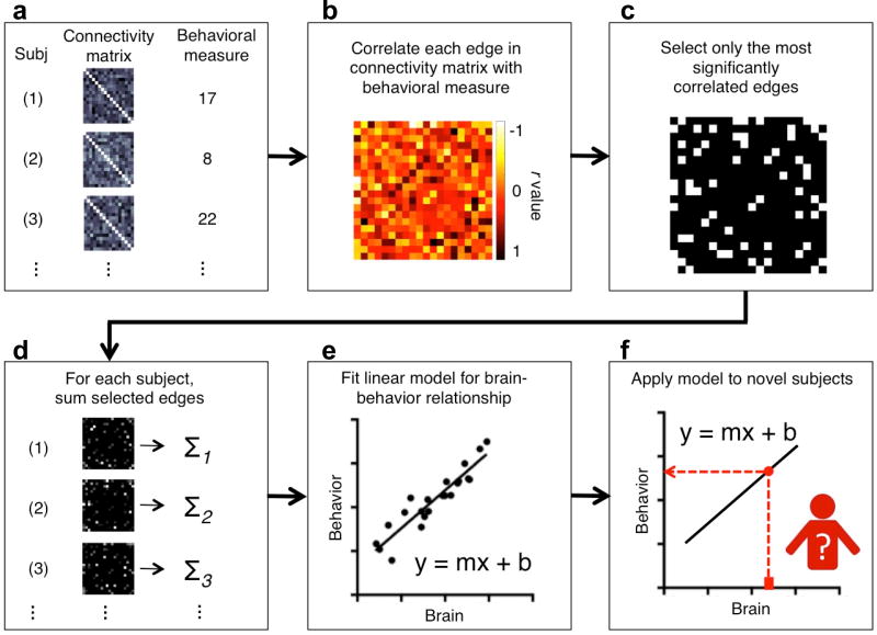
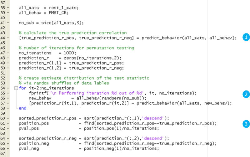
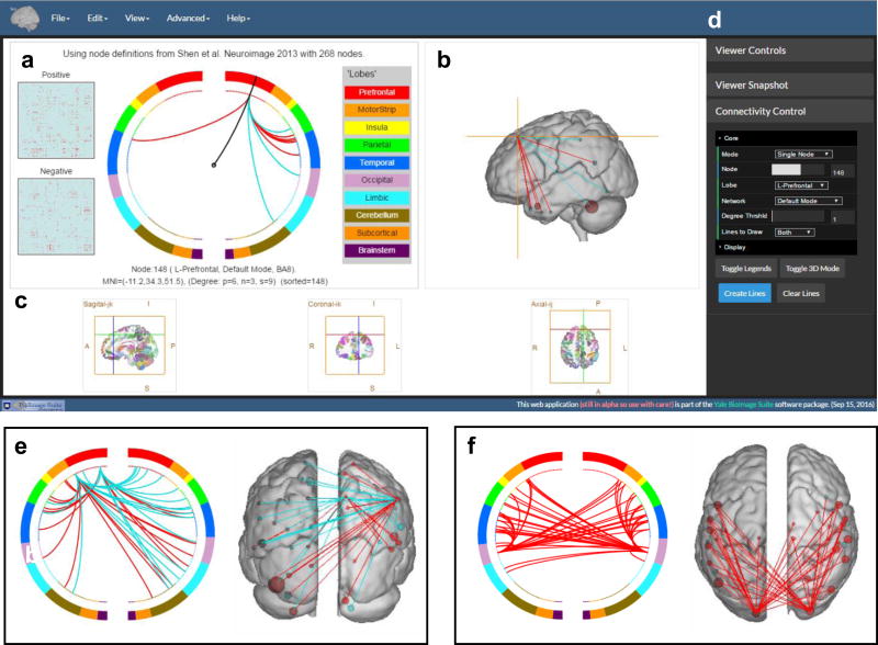
Neuroimaging is a fast-developing research area in which anatomical and functional images of human brains are collected using techniques such as functional magnetic resonance imaging (fMRI), diffusion tensor imaging (DTI), and electroencephalography (EEG). Technical advances and large-scale data sets have allowed for the development of models capable of predicting individual differences in traits and behavior using brain connectivity measures derived from neuroimaging data. Here, we present connectome-based predictive modeling (CPM), a data-driven protocol for developing predictive models of brain-behavior relationships from connectivity data using cross-validation. This protocol includes the following steps: (i) feature selection, (ii) feature summarization, (iii) model building, and (iv) assessment of prediction significance. We also include suggestions for visualizing the most predictive features (i.e., brain connections). The final result should be a generalizable model that takes brain connectivity data as input and generates predictions of behavioral measures in novel subjects, accounting for a considerable amount of the variance in these measures. It has been demonstrated that the CPM protocol performs as well as or better than many of the existing approaches in brain-behavior prediction. As CPM focuses on linear modeling and a purely data-driven approach, neuroscientists with limited or no experience in machine learning or optimization will find it easy to implement these protocols. Depending on the volume of data to be processed, the protocol can take 10-100 min for model building, 1-48 h for permutation testing, and 10-20 min for visualization of results.


Figures

Figure 1
Figure 1. Schematic of connectome-based predictive modeling (CPM)
a) For each subject, inputs to CPM are a connectivity matrix and behavioral measures. Connectivity matrices can be from several different modalities and behavioral measures should have a sufficient dynamic range or spread across subjects to support prediction in novel data. The input data needs to be divided into a training set and a testing set. Procedure step 1, 2. b) Across all subjects in the training set, each edge in the connectivity matrices is related to the behavioral measures using a form of linear regression, including Pearson correlation, Spearman correlation, or robust regression. Procedure step 3. c) After linear regression, the most important edges are selected for further analysis. Typically, important edges are selected using significance testing, though other strategies exist, e.g. selecting edges whose correlation value is above a pre-defined threshold. Procedure step 4. d) For each subject, the most important edges are then summarized into a single subject value. Usually, the edge strengths are simply summed. Procedure step 5. e) Next a predictive model is built assuming a linear relationship between the single-subject summary value of connectivity data (independent variable) and the behavioral variable (the dependent variable). Procedure step 6. f) Next, summary values are calculated for each subject in the testing set. This value is then input into the predictive model. The resulting value is the predicted behavioral measure for the current test subject. Procedure step 7.
Figure 2
Figure 2. Visualizing selected connectivity features
These illustrations were created using BioImage Suite1 (https://www.nitrc.org/projects/bioimagesuite/). a) Glass brain plots: each node is represented as a sphere, where the size of the sphere indicating the number of edges emanating from that node. The set of positive features (edges) is coded red and the set of negative features (edges) is coded blue. b) Circle plots: nodes are arranged in two half circles approximately reflecting brain anatomy from anterior (top of the circle, 12 o’clock position) to posterior (bottom of the circle, 6 o’clock position), and the nodes are color coded according to the cortical lobes. Positive and negative features (edges) are drawn between the nodes on separate plots. The lobes are prefrontal (PFC), motor (MOT), insula (INS), parietal (PAR), temporal (TEM), occipital (OCC), limbic (LIM), cerebellum (CER), subcortical (SUB), brain stem (BSM). c) Matrix plots: rows and columns represent pre-defined networks (usually includes multiple nodes). The cells represent the difference between the total number of positive edges and the total number of negative edges connecting the nodes in the two networks.
Figure 3
Figure 3. Example CPM code for step 1–3
a) (1) Load connectivity matrices and behavioral data into memory. (2) Divide data into training and testing sets for cross validation. In this example, leave-one-out cross-validation is used. (3) Relate connectivity to behavior. In this example, Pearson correlation is used. Note that the code outlined with a red box in (a) may be replaced with any of three alternatives in the right hand panels: b) rank (Spearman) correlation; c) partial correlation; d) robust regression.
Figure 4
Figure 4. Example CPM code for steps 4–8
a) (4) Edge selection. In this example, a significance threshold of p=0.01 is used (see line 42 in Fig. 2: “thresh=0.01”). Alternatively, a sigmoidal weighting function may be used by replacing the code in the green box with the code provided in (b). (5) Forming single-subject summary values. For each subject in the training set, the selected edges are then summarized to a single value per subject for the positive edge set and the negative edge set separately. (6) Model fitting. In this example, a linear model (Y=mX+b) is fitted for the positive edge set and the negative edge set, separately. Alternatively, a model combining both terms may be used by replacing the code in the red box with the code provided in (c). Circle (7) Prediction in novel subjects. Single subject summary values are calculated for each subject the testing set and are used as an input to the predictive model (equation) estimated in Step 6. The resulting value is the predicted behavioral measure for the current subject. Circle (8) Evaluation of predictive model. Correlation and linear regression between the predicted values and true values provide measures to evaluate prediction performance. Alternatively, the predictive model may also be evaluated using mean squared error by replacing the code in the blue box with the code provided in (d).
Figure 5
Figure 5. Example permutation test code for steps 9–11
(1) Calculate the true prediction correlation. (2) Shuffle data labels, calculate correlation coefficient, and repeat for 100–10,000 iterations. (3) Calculate p-values.
Figure 6
Figure 6. Online visualization tool for making circle plots and glass brain plots described in steps 12–15
The tool can be accessed via the link http://bisweb.yale.edu/connviewer/. The user interface includes four panels, a) displays the circle plot and relevant information of a selected node. b) displays the 3D view of a glass MNI brain that can be rotated using a mouse. c) displays three orthogonal views of the brain parcellation from Shen et al with color coded nodes overlaid on top of an MNI brain. d) displays the set of control modules including “Viewer Controls”, “Viewer Snapshot” and “Connectivity Control”. The “Connectivity Control” module is expanded and the six filters under “core” are shown with specified parameters. All three circle plots and glass brain plots in a), b), e) and f) are generated using the sample matrices. Edges in the sample matrices are generated randomly and the matrices are pre-loaded when the tool initializes. Circle plot and glass brain plot in a) and b) are created by setting “mode = single node”, “node =148” and “lines to draw = both”. Circle plot and glass brain plot in e) are created by setting “mode = single lobe”, “lobe = R-Prefontal”, “Degree thrshld = 15”, “Lines to draw = both”. Circle plot and glass brain plot in f) are created by setting “mode = single network”, “network = visual”, “Degree thrshld = 35”, “Lines to draw = positive”.

Similar articles

Cited by

References

    1. Kriegeskorte N, Simmons WK, Bellgowan PS, Baker CI. Circular analysis in systems neuroscience: the dangers of double dipping. Nat. Neurosci. 2009;12:535–540. - PMC - PubMed
    1. Vul E, Harris C, Winkielman P, Pashler H. Puzzlingly high correlations in fMRI studies of emotion, personality, and social cognition. Perspect. Psychol. Sci. 2009;4:274–290. - PubMed
    1. Gabrieli JD, Ghosh SS, Whitfield-Gabrieli S. Prediction as a humanitarian and pragmatic contribution from human cognitive neuroscience. Neuron. 2015;85:11–26. doi: 10.1016/j.neuron.2014.10.047. - DOI - PMC - PubMed
    1. Finn ES, et al. Functional connectome fingerprinting: identifying individuals using patterns of brain connectivity. Nat Neurosci. 2015 doi: 10.1038/nn.4135. - DOI - PMC - PubMed
    1. Rosenberg MD, et al. A neuromarker of sustained attention from whole-brain functional connectivity. Nat Neurosci. 2016;19:165–171. doi: 10.1038/nn.4179. - DOI - PMC - PubMed

Publication types