Spontaneous activity in the piriform cortex extends the dynamic range of cortical odor coding

Abstract

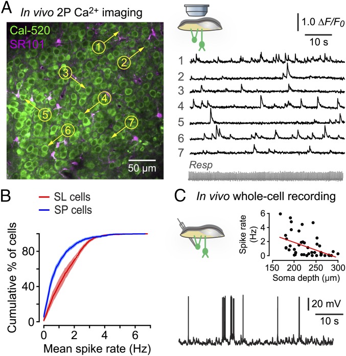
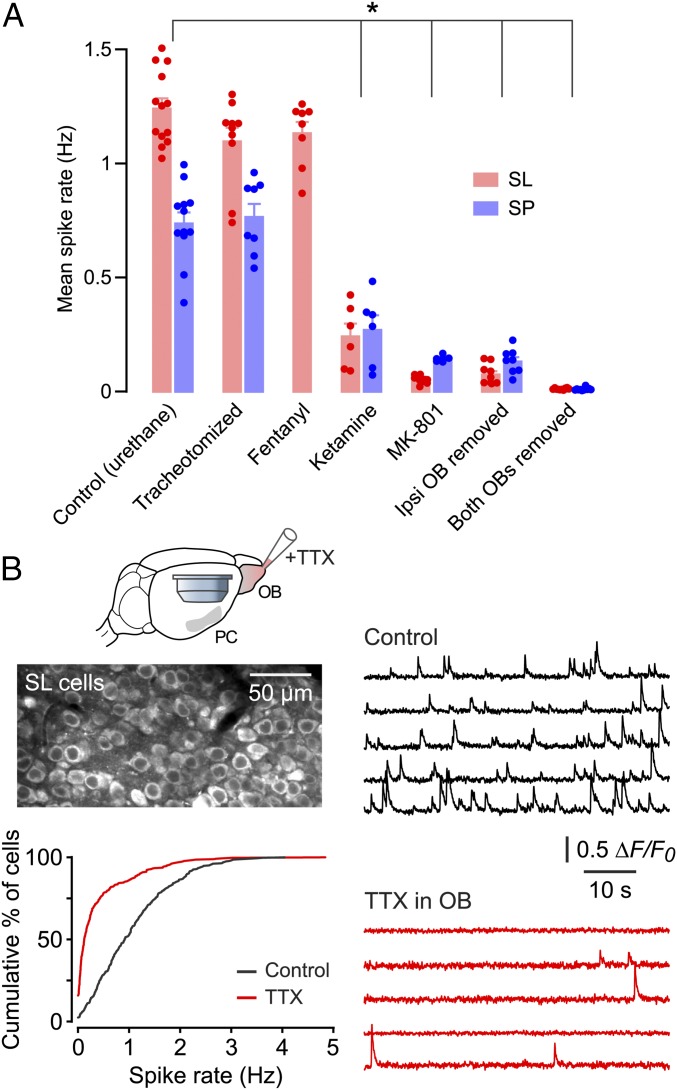
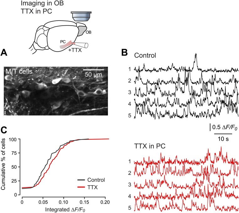
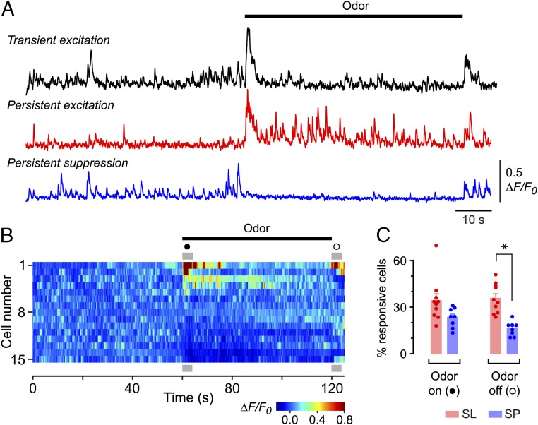
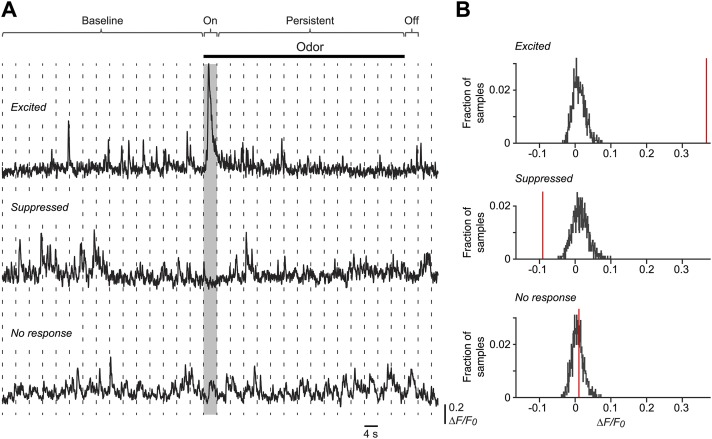
Neurons in the neocortex exhibit spontaneous spiking activity in the absence of external stimuli, but the origin and functions of this activity remain uncertain. Here, we show that spontaneous spiking is also prominent in a sensory paleocortex, the primary olfactory (piriform) cortex of mice. In the absence of applied odors, piriform neurons exhibit spontaneous firing at mean rates that vary systematically among neuronal classes. This activity requires the participation of NMDA receptors and is entirely driven by bottom-up spontaneous input from the olfactory bulb. Odor stimulation produces two types of spatially dispersed, odor-distinctive patterns of responses in piriform cortex layer 2 principal cells: Approximately 15% of cells are excited by odor, and another approximately 15% have their spontaneous activity suppressed. Our results show that, by allowing odor-evoked suppression as well as excitation, the responsiveness of piriform neurons is at least twofold less sparse than currently believed. Hence, by enabling bidirectional changes in spiking around an elevated baseline, spontaneous activity in the piriform cortex extends the dynamic range of odor representation and enriches the coding space for the representation of complex olfactory stimuli.

Keywords: anesthetic; calcium imaging; in vivo; olfaction; two-photon.

Fig. S1.

Glutamatergic neuronal types and schematic diagram of excitatory circuits in the mouse anterior PC. (A) Reconstructed dendritic arbors of an SL cell (Left) and an SP cell (Right) showing the approximate location of their somas in layer 2. Glutamatergic cells (notably, deep pyramidal cells) are also present at lower density in layer 3 but are not shown here. (B) Schematic of simplified excitatory circuits (Left) and cytoarchitecture (Right). SL cells receive stronger afferent (Aff) input than SP cells but much weaker associational (Assn) input.

Fig. 1.

The PC is spontaneously active in vivo. (A) Cal-520–labeled SL cell somas (Left) and corresponding ∆F/F₀ fluorescence traces from the numbered cells (Right) showing spontaneous activity. Resp, simultaneously recorded respiration. SR 101 labels astrocytes. (B) Averaged cumulative histograms showing that the mean spontaneous spike rate in SL cells (n = 7 mice, 1,928 cells) and SP cells (n = 6 mice, 1,005 cells; shaded regions are ± SEM) are significantly different (P < 0.0001, Kolmogorov–Smirnov test). (C) A typical in vivo whole-cell recording showing spontaneous spiking in an SL cell (depth 166 µm). (Inset) The spontaneous spike rate was higher in the more superficial SL cells (soma depth 160–230 µm, 1.7 ± 0.3 Hz; mean ± SEM) than in the deeper SP cells (230–300 µm, 0.7 ± 0.2 Hz; mean ± SEM, P = 0.005, Mann–Whitney test) and was negatively correlated with recording depth (r = 0.47, P = 0.0006, n = 50 cells from 48 mice; F test on linear regression).

Fig. S2.

Calibration procedure for converting measured calcium transients to spike number. (A, Upper) Simultaneous two-photon Ca²⁺ imaging and cell-attached recording in vivo from a Cal-520–labeled SL cell. The pipette solution contained Alexa-Fluor 594 (50 µM). (Lower) Typical ∆F/F₀ trace and corresponding spikes recorded via the patch electrode. (B) Plot of integrated ∆F/F₀ versus the number of simultaneously recorded spikes. Each color indicates data from a different neuron (n = 22 data points from three cells from two mice). A straight line fitted to all data points had a slope of 73 ± 1 spikes per unit area under the ∆F/F₀ waveform (mean ± SD, R² > 0.98).

Fig. S3.

Identification of GABAergic interneurons confirms that most of the neurons imaged in layer 2 are glutamatergic (SL and SP cells). Furthermore, interneurons in layer 2 also exhibit spontaneous activity. (A) Typical image of neurons in layer 2a loaded with the red-shifted calcium indicator Cal-590 AM in a urethane-anesthetized transgenic GAD67-GFP mouse. Interneurons (green) are scarce (approximately 4% of the total number of neurons), confirming a previous report (28). Similar results were obtained in layer 2b. (B) Typical ∆F/F₀ traces (Lower) showing spontaneous activity in two identified interneurons (Upper, arrowheads). (C) Cumulative histogram showing the spontaneous spike rate of interneurons in layer 2a or layer 2b (2a: mean 0.35 ± 0.07 Hz, n = 28 cells; 2b: 0.14 ± 0.03 Hz, n = 33 cells; P = 0.065, Kolmogorov–Smirnov test). The spike rate was calibrated using a different method from that shown in Fig. S2 for Cal-520 AM. See SI Materials and Methods for details.

Fig. 2.

Properties of spontaneous spiking in SL and SP cells under different experimental conditions. (A) Each data point is the averaged firing rate for all cells (n approximately 60–230 cells) in a field of view in a single experiment. Bars show mean ± SEM of the points. *P < 0.05 (one-way ANOVA with Tukey’s post hoc test, comparing control with other conditions in SL cells and SP cells separately). SP cells were not imaged in fentanyl. (B, Upper Left) Imaged field of SL cells in this experiment (using Cal-520). (Right) ∆F/F₀ traces for the same five SL cells recorded before (control, Upper) and during (Lower) the superfusion of TTX over the ipsilateral OB. (Lower Left) Cumulative histograms of spontaneous spike rates recorded in this experiment before (black trace) and during (red trace) TTX application. P < 0.0001 (n = 368 cells, Kolmogorov–Smirnov test).

Fig. S4.

Pharmacological silencing of the PC has no effect on spontaneous spiking in the ipsilateral OB. (A, Upper) Schematic of the imaging of M/T cells in the OB using the genetically encoded indicator GCaMP6f while activity in the ipsilateral anterior PC was silenced by superperfusing TTX through a craniotomy made over the PC. (Lower) A typical field of view. (B) Representative ∆F/F₀ traces showing spontaneous activity measured simultaneously in the same population of five M/T cells before (black traces) and during (red traces) the application of TTX. (C) Cumulative histograms of integrated ΔF/F₀ in M/T cells before (black trace) and during (red trace) TTX application to the ipsilateral anterior PC. There was no significant difference in spontaneous activity (n = 93 M/T cells, P = 0.11, Kolmogorov–Smirnov test).

Fig. 3.

Odors both excite and suppress spiking activity. (A) ∆F/F₀ recordings from three different layer 2 cells showing the typical diversity of odor responses. The indicator was Cal-520. (B) Color raster plot of ∆F/F₀ in a selected subset of SL cells in one experiment, ranked by their peak ∆F/F₀ during the first 4 s after odor application. Gray bars designate 4 s after odor onset (●) and offset (O). (C) Percentages of SL and SP cells that were responsive (i.e., were either excited or suppressed) during odor onset or offset. Bars show mean ± SEM of the individual experiments (points). *P < 0.001 (n = 10 SL and n = 8 SP experiments, unpaired two-tailed t test).

Fig. S5.

Method for finding whether a cell is excited or suppressed by odor. (A) Representative ∆F/F₀ traces of cell somas with significant responses (Top, excited; Middle, suppressed) or with no response (Bottom) during the first 4 s of odor presentation (on response; gray box). The significance of these responses was estimated using a bootstrapping procedure as described in SI Materials and Methods. Briefly, the ∆F/F₀ traces were divided into 4-s segments (dashed vertical lines), each containing 120 frames; then the ∆F/F₀ values for each cell soma were bootstrapped 500 times for each segment, and a histogram of these values was calculated. The histograms for all fifteen 4-s segments during the 60-s baseline period were averaged to yield an average background distribution for each cell; examples of these for three different cells are shown in B. A similar procedure was used for the 4-s on and off periods (except that no averaging was done) and for the 56-s persistent period. (B) Results of the analysis for the cells shown in A. Histograms around zero are the averaged ∆F/F₀ values of the baseline period, and the red vertical line indicates the median of the distribution of bootstrapped ∆F/F₀ values measured in the 4-s odor-on test period. The cell was scored as excited if the median was above the 99.9th percentile of the baseline distribution (Top), as suppressed if the median was below the 0.1th percentile (Middle), and otherwise was scored as showing no response (Bottom). A similar analysis was done for the 4-s odor-off period.

Fig. S6.

SL and SP cells differ significantly in the percentages that are excited or suppressed by odor, but only at the odor-off period. In addition, changing the odor concentration has little effect on the percentages of SL cells that are excited or suppressed by the odor. (A) Percentages of SL cells (red) and SP cells (blue) that are excited (E) or suppressed (S) at either the onset or offset of a 60-s application of the odor. Colored bars and error bars indicate mean ± SEM. Filled circles indicate the percentage of responsive cells measured in each experiment. *P < 0.05 (n = 10 SL and n = 8 SP experiments, unpaired two-tailed t test). (B, Upper) Output of the photo ionization device (PID). Five consecutive trials are shown (gray traces, all overlapping and indistinguishable), together with their average (blue trace). These data show that odor pulses are reproducible and that odor concentration does not decline during the 60-s application period. (Lower) Log-log plot of PID output versus dilution factor for two odorants, confirming dilution. (C) Percent of SL cells that are excited (Left) or suppressed (Right) by two different odorants (amyl acetate, yellow; ethyl butyrate, black) applied at three different dilutions. Measurements were made in three different time periods: on, i.e., the first 4 s after odor onset; off, i.e., the first 4 s after odor offset; persistent, a period from 4–60 s after odor onset. Symbols and error bars indicate mean ± SEM. For each time period and each odorant, the percentage of responsive cells was not significantly different among the three odor concentrations (n = 4 experiments per data point, one-way ANOVA).

Fig. S7.

The spike rate, averaged over the population of SL and SP cells, shows only transient increases at odor onset and offset. (A) Mean population spike rate in clean air (first 60 s) and in odor (60–120 s) in SL cells (Upper, n = 10 imaged fields) and SP cells (Lower, n = 8 imaged fields). Odor onset and offset are labeled with filled and open symbols, respectively. Shading indicates ± SEM. (B) Spike rate averaged over either the 60-s clean-air baseline period or the subsequent 60-s period of odor application, for SL cells (Upper) and SP cells (Lower). Each pair of symbols shows the average from a single imaged field of view (the same dataset as in A). The mean rate was not significantly different between the two time windows (n = 10 SL and n = 8 SP experiments, paired two-tailed t test).

Fig. 4.

Properties of odor-evoked excitation and suppression. (A) Each point shows the peak odor-evoked response in an odor-excited neuron plotted versus the mean spontaneous spike rate measured in the same neuron. Different colors indicate different odors. Superimposed straight lines indicate a correlation for SP cells (slope = 0.25, correlation coefficient = 0.48, n = 83 cells) but not for SL cells (slope = 0.02, correlation coefficient = 0.07, n = 321 cells). (B, Left) Imaged field of SL cells with somatic ROIs outlined. The other three panels show the same ROIs with color-coded odor responses to the three odors indicated. The indicator was GCaMP6f. (C) Each red point indicates the mean distance between each excited cell in an imaged field and its five nearest neighbors that also were excited, averaged across all excited cells in that field. Blue points show the same measure for suppressed cells. Lines connect data from the same experiment (n = 10 experiments for SL cells, n = 8 experiments for SP cells). In three SP cell experiments (red points without connected blue points) there were fewer than six suppressed cells in the imaged field. ns, not significant (P > 0.5, unpaired two-tailed t test).

Fig. S8.

The mean distances between odor-excited and odor-suppressed SL or SP cells are similar, suggesting that excited and suppressed cells are randomly intermingled. (A) The red points in this panel are the same as those in Fig. 4C of the main text and show the mean distance between each excited (E) cell in an imaged field and its five nearest neighbors that were also excited, averaged across all excited cells in that field (n = 10 experiments for SL cells; n = 8 experiments for SP cells). In contrast to Fig. 4C, the blue points in this panel show the mean distance between each excited cell and its five nearest neighbors that were suppressed (S) by odor (not to be confused with the blue points in Fig. 4C, which show distances between suppressed cells.) Lines connect data from the same experiment. Mean distances are not significantly different for SL and SP cells (SL: 60.3 ± 5.7 µm for E–E, 57.9 ± 5.2 µm for E–S, mean ± SEM, n = 10, P = 0.77; SP: 116.1 ± 15.2 µm for E–E, 118.1 ± 8.0 µm for E–S, n = 8, P = 0.91; unpaired two-tailed t test). (B) As in A, except that the points now show the mean distance from each suppressed cell to its five nearest-neighbor excited cells (red points) or suppressed cells (blue points). In three SP cell experiments (red points without connected blue points) there were fewer than six suppressed cells in the imaged field. Mean distances are not significantly different for SL and SP cells (SL: 56.7 ± 6.3 µm for S–E, 63.7 ± 7.7 µm for S–S, n = 10, P = 0.49; SP: 94.6 ± 12.7 µm for S–E, n = 8, 98.5 ± 24.3 µm for S–S, n = 5, P = 0.88; unpaired two-tailed t test). Finally, the mean distance from each excited cell to its neighbors (both excited and suppressed) was not significantly different from the mean distance from each suppressed cell to its neighbors (dashed lines connecting panels A and B; SL: P = 0.85; SP: P = 0.14; unpaired two-tailed t test). ns, not significant.

References

1. Raichle ME. The restless brain: How intrinsic activity organizes brain function. Philos Trans R Soc Lond B Biol Sci. 2015;370(1668):20140172. - PMC - PubMed
1. Barth AL, Poulet JF. Experimental evidence for sparse firing in the neocortex. Trends Neurosci. 2012;35(6):345–355. - PubMed
1. Brette R. Philosophy of the spike: Rate-based vs. spike-based theories of the brain. Front Syst Neurosci. 2015;9:151. - PMC - PubMed
1. Luczak A, McNaughton BL, Harris KD. Packet-based communication in the cortex. Nat Rev Neurosci. 2015;16(12):745–755. - PubMed
1. McGinley MJ, et al. Waking state: Rapid variations modulate neural and behavioral responses. Neuron. 2015;87(6):1143–1161. - PMC - PubMed
Publication types
MeSH terms
Substances
LinkOut - more resources