Two dynamic regimes in the human gut microbiome

Abstract

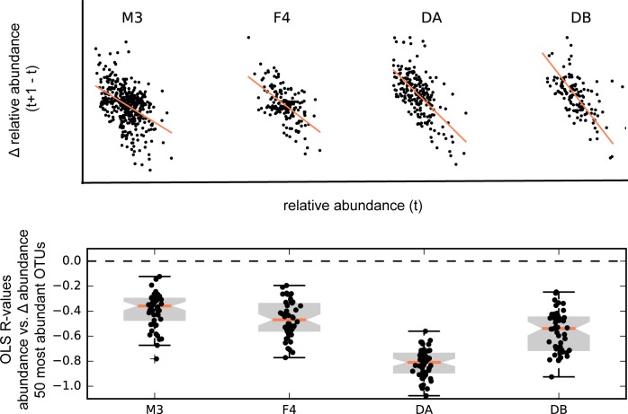
The gut microbiome is a dynamic system that changes with host development, health, behavior, diet, and microbe-microbe interactions. Prior work on gut microbial time series has largely focused on autoregressive models (e.g. Lotka-Volterra). However, we show that most of the variance in microbial time series is non-autoregressive. In addition, we show how community state-clustering is flawed when it comes to characterizing within-host dynamics and that more continuous methods are required. Most organisms exhibited stable, mean-reverting behavior suggestive of fixed carrying capacities and abundant taxa were largely shared across individuals. This mean-reverting behavior allowed us to apply sparse vector autoregression (sVAR)-a multivariate method developed for econometrics-to model the autoregressive component of gut community dynamics. We find a strong phylogenetic signal in the non-autoregressive co-variance from our sVAR model residuals, which suggests niche filtering. We show how changes in diet are also non-autoregressive and that Operational Taxonomic Units strongly correlated with dietary variables have much less of an autoregressive component to their variance, which suggests that diet is a major driver of microbial dynamics. Autoregressive variance appears to be driven by multi-day recovery from frequent facultative anaerobe blooms, which may be driven by fluctuations in luminal redox. Overall, we identify two dynamic regimes within the human gut microbiota: one likely driven by external environmental fluctuations, and the other by internal processes.

Fig 1. Time series stationarity and non-stationarity.

Grey lines depict time series, with the mean plotted in red. The top left time series is stationary, with a stable mean (i.e. mean-reverting) and variance (i.e. non-heteroskedastic). The top right trace shows a non-stationary time series where the mean and variance change monotonically. The bottom left trace shows a time series with non-stationary variance (i.e. a sudden bloom event). The bottom right trace shows a non-stationary time series with both a changing variance and a non-monotonically changing mean.

Fig 2. Flow chart indicating what time series modeling approach is appropriate given the structure of a data set.

Fig 3. Two dynamic regimes in the gut microbiome.

The top panel shows the relative abundance trace for an OTU. The second panel shows the same time series after first-differencing (i.e. taking the derivative to obtain the rate). In this data set, first-differencing ensured that each time series was stationary and appropriate for sparse vector autoregressive (sVAR) modeling. The third row of plots shows autoregressive and non-autoregressive rate dynamics, based on fitting the sVAR model. Autoregressive model coefficients (bottom left) provide information on time-lagged interactions between OTUs within the model (i.e. equivalent to partial Granger coefficients). OTU-OTU covariance (bottom right) of non-autoregressive dynamics provides information on co-fluctuating taxa.

Fig 4. Alpha diversity is correlated with conditionally rare taxa (CRT) blooms.

Black lines show the Shannon effective number of species (i.e. N_eff, a measure of alpha diversity) for each time series used in this analysis. The red dashed lines show the average N_eff for each time series. The average N_eff is between 28–51 across the time series, which is high enough that compositional effects are expected to be negligible (Freidman and Alm, 2012). Major perturbations in alpha diversity are associated with CRT blooms (orange lines = sum of CRT abundances).

Fig 5. Autocorrelation decay plots for the 50 most abundant OTUs in each time series.

Each black line represents the autocorrelation for a single OTU over different time lags (in days). The top row of plots shows autocorrelation (y-axis) for up to 50-day lags (x-axis). Orange dashed lines indicate an autocorrelation coefficient of 0.0. Dashed grey lines show the zoom-in region from the upper row of plots presented in the second row of plots (lags up to 10 days).

Fig 6. OTUs in the time series data show a propensity for mean-reversion.

The top row of plots shows the change in relative abundance from time t to time t+1 (y-axis) vs. the relative abundance (x-axis) for OTU 850870 (Greengenes ID; Bacteroides spp.; the most abundant OTU in M3, F4 and DB time series and 2^nd most abundant OTU in DA time series). The bottom plot summarized the ordinary least-squares (OLS) regression coefficient (R) for the top 50 most abundant OTUs from each data set. In general, there is a negative association between an OTU’s change in abundance and its current abundance level, suggesting that OTUs have fixed carrying capacities. The average magnitude of the regression coefficient appears to be an indicator of the returning force. These results are consistent with stationarity.

Fig 7

(A) shows decay in the number of Dirichelet multinomial mixture model (DMM) states as the sparcity of the time series is increased for the top 50 most abundant OTUs from each time series and for the 76 abundant OTUs shared across all four time series. The plateau is at 6 states for both methods (grey dashed line). (B) shows state classifications for samples taken from all four individuals (top 50 OTUs from each time series sampled at every 11^th time point). States are largely unique to individuals (i.e. colors indicate unique states), with the exception of a single time point in the DA series that was assigned to a state (blue) that is dominant in DB.

Fig 8. Scatter plots of the log median abundances of shared 99% OTUs across time series.

Taxa that are present across time series show a positive correlation in their median abundances.

Fig 9. Amount of variance explained by sVAR(3) model for top 50 OTUs in each time series.

Bars are colored by order: blue = Bacteroidales, red = Clostridiales, black = Enterobacteriales, pink = Verrucomicrobiales, yellow = Erysipelotrichales, olive = Bifidobacteriales, silver = Pasteurellales, cyan = Synergistales.

Fig 10. Granger causal networks for each time series.

Trees show phylogenetic relationships between taxa. Edges are interactions identified in the sVAR(3) model that also show significant Granger causality (p < 0.05). Symbols indicate oxygen tolerance and growth traits. CRT stands for ‘conditionally rare taxon’, which is defined by a coefficient of bimodality > 0.8 and a maximum abundance of > 10% of the community. CRTs are organisms that are usually rare, but occasionally bloom to very high abundance. CRTs tend to be facultative aerobes, or aerotolerant taxa.

Fig 11. Phylogenetic relatedness corresponds to similarity in dynamics for top 50 most abundant OTUs.

Each plot is a heatmap showing the density of pairwise OTU-OTU correlation or sVAR coefficients (y-axes) vs. pairwise phylogenetic distances (x-axes). The red lines show the mean coefficient along phylogenetic distance windows. Top row shows Spearman correlations calculated based on raw count data. Second row shows Spearman correlations calculated based on the first-difference (delta) of the count data. The third row shows the Spearman correlations performed on the residuals of a sVAR(3) model fit to the deltas. The bottom row shows the sVAR(3) coefficients. The heatmap colors denote the density of OTU-OTU pairs at a given hexagonal pixel on the plot.

References

1. Turnbaugh PJ, Ley RE, Hamady M, Fraser-Liggett CM, Knight R, Gordon JI. The Human Microbiome Project. Nature. 2007;449(7164):804–10. 10.1038/nature06244 - DOI - PMC - PubMed
1. Lax S, Smith DP, Hampton-Marcell J, Owens SM, Handley KM, Scott NM, et al. Longitudinal analysis of microbial interaction between humans and the indoor environment. Science. 2014;345(6200):1048–52. 10.1126/science.1254529 - DOI - PMC - PubMed
1. Fierer N, Lauber CL, Zhou N, McDonald D, Costello EK, Knight R. Forensic identification using skin bacterial communities. Proc Natl Acad Sci USA. 2010;107(14):6477–81. 10.1073/pnas.1000162107 - DOI - PMC - PubMed
1. Franzosa EA, Huang K, Meadow JF, Gevers D, Lemon KP, Bohannan BJ, et al. Identifying personal microbiomes using metagenomic codes. Proc Natl Acad Sci USA. 2015;112(22):E2930–E8. 10.1073/pnas.1423854112 - DOI - PMC - PubMed
1. Bakken JS, Borody T, Brandt LJ, Brill JV, Demarco DC, Franzos MA, et al. Treating Clostridium difficile infection with fecal microbiota transplantation. Clin Gastroenterol Hepatol. 2011;9(12):1044–9. 10.1016/j.cgh.2011.08.014 - DOI - PMC - PubMed
Publication types
LinkOut - more resources