Mindboggling morphometry of human brains

Abstract

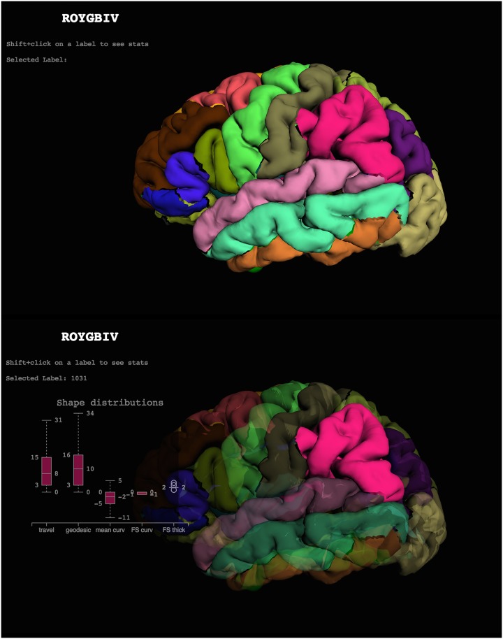
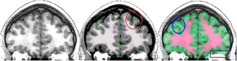
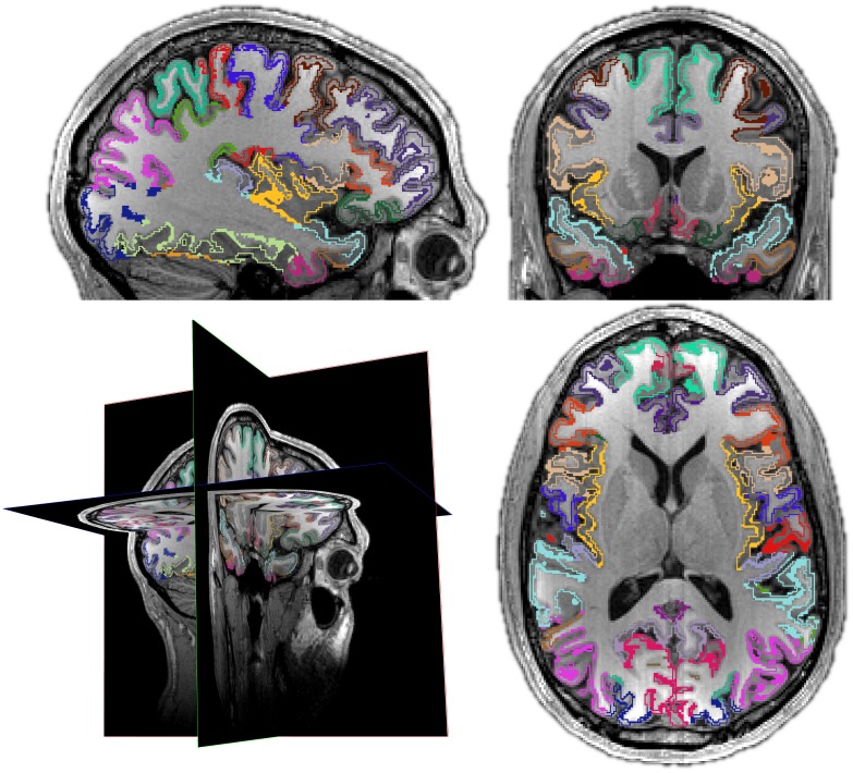
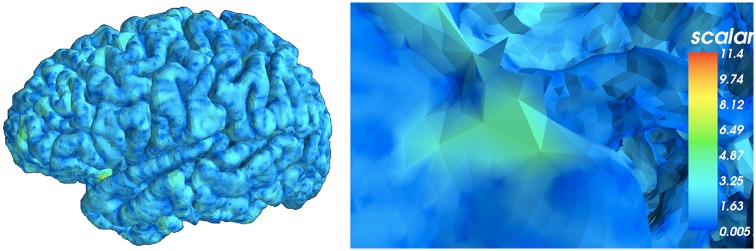
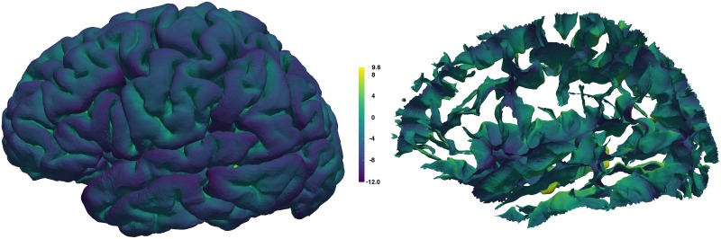
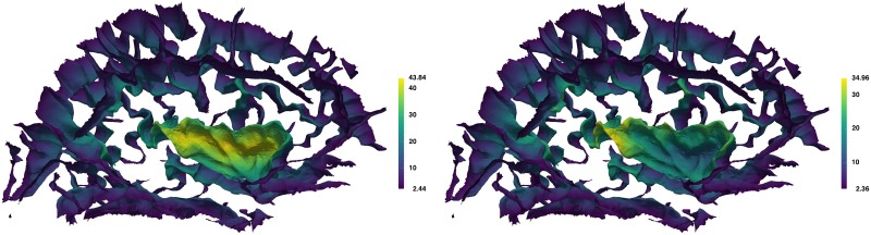
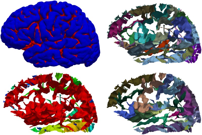
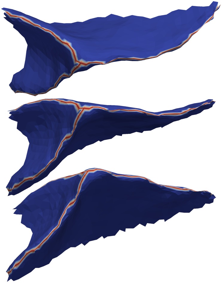
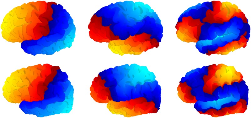
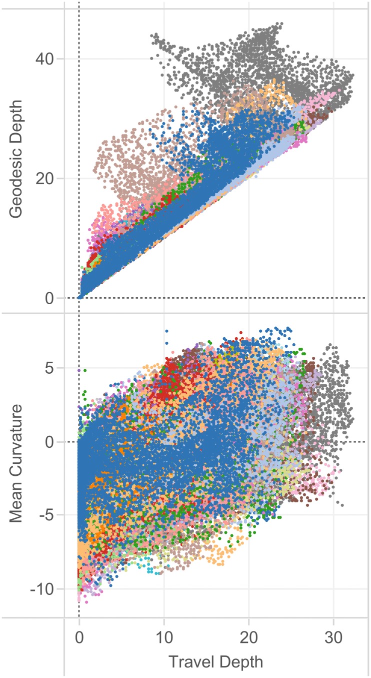
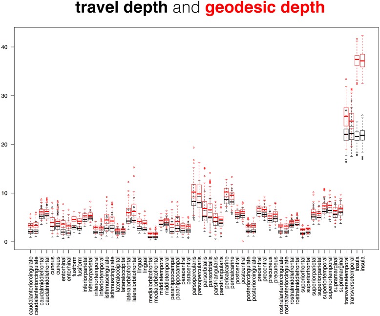
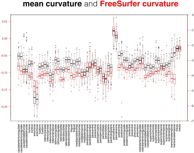
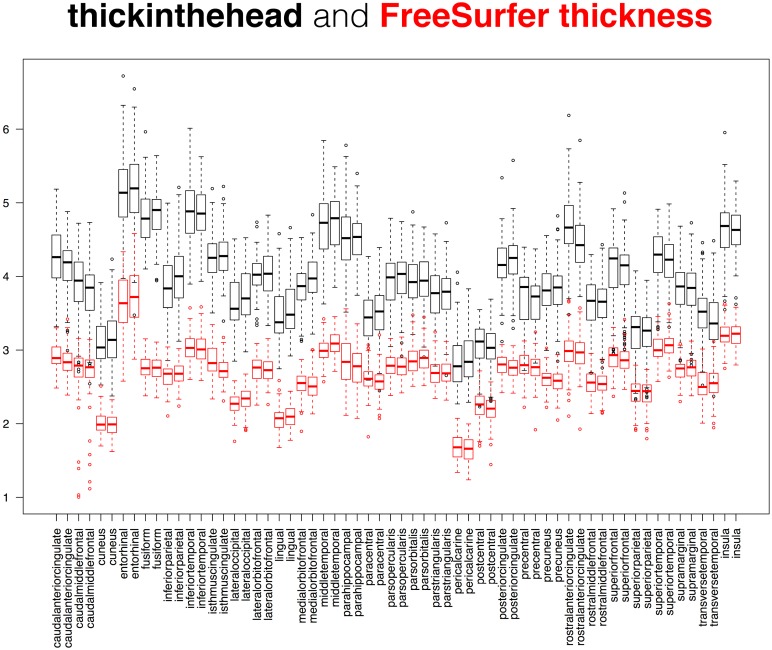
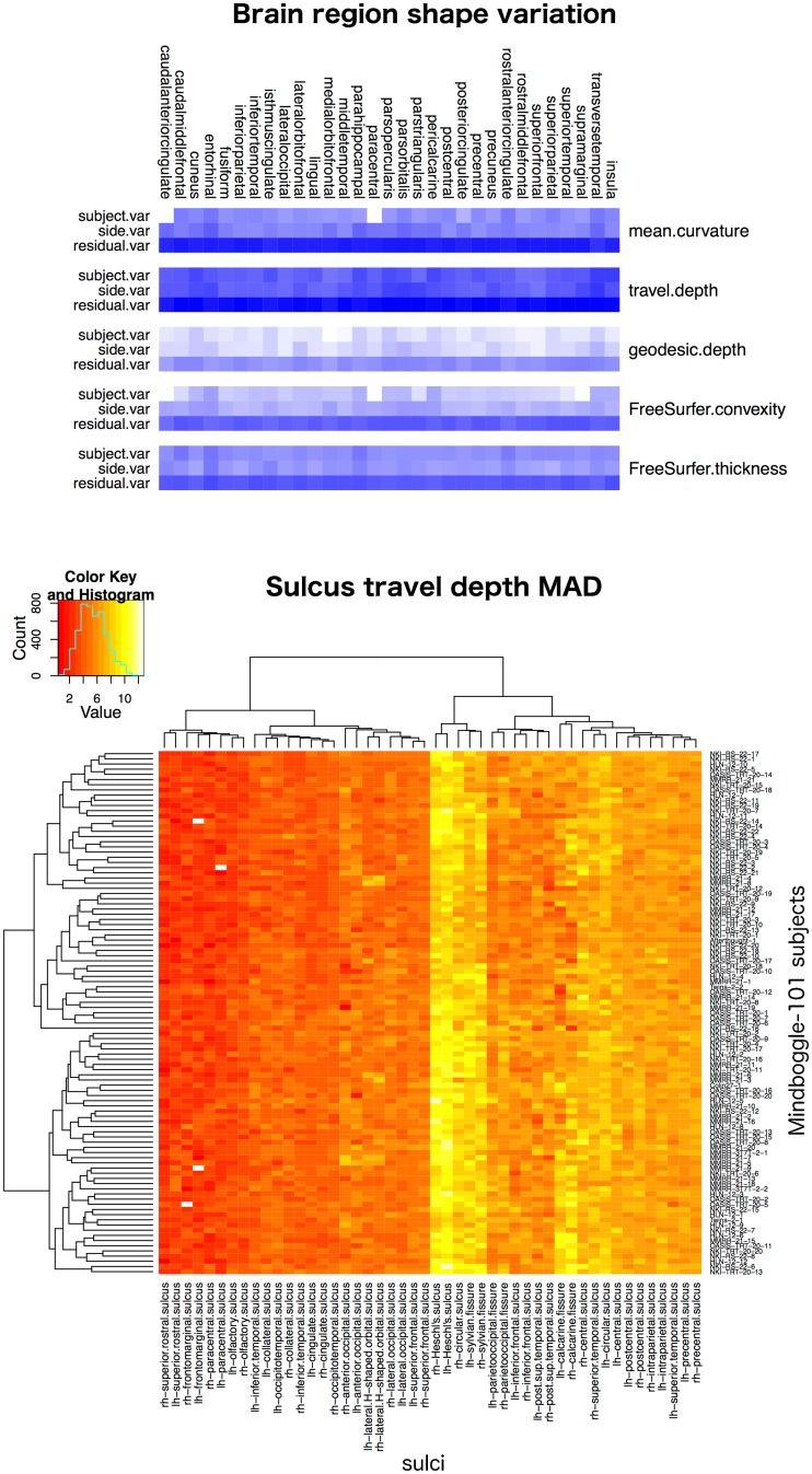
Mindboggle (http://mindboggle.info) is an open source brain morphometry platform that takes in preprocessed T1-weighted MRI data and outputs volume, surface, and tabular data containing label, feature, and shape information for further analysis. In this article, we document the software and demonstrate its use in studies of shape variation in healthy and diseased humans. The number of different shape measures and the size of the populations make this the largest and most detailed shape analysis of human brains ever conducted. Brain image morphometry shows great potential for providing much-needed biological markers for diagnosing, tracking, and predicting progression of mental health disorders. Very few software algorithms provide more than measures of volume and cortical thickness, while more subtle shape measures may provide more sensitive and specific biomarkers. Mindboggle computes a variety of (primarily surface-based) shapes: area, volume, thickness, curvature, depth, Laplace-Beltrami spectra, Zernike moments, etc. We evaluate Mindboggle's algorithms using the largest set of manually labeled, publicly available brain images in the world and compare them against state-of-the-art algorithms where they exist. All data, code, and results of these evaluations are publicly available.

Fig 1. Cortical labels displayed in the ROYGBIV interactive online brain image viewer.

The anatomical labels included in the DKT cortical labeling protocol [22] used to label the Mindboggle-101 data are displayed on a left cortical surface. These two panels show the current state of our prototype for a browser-based interactive visualization of the left hemisphere of a human brain [70] and accompanying plot of some of Mindboggle’s shape measures for a selected region (http://roygbiv.mindboggle.info).

Fig 2. FreeSurfer and ANTs gray/white matter segmentation.

Left: Coronal slice of a T1-weighted brain MRI. Middle: Cross-section of FreeSurfer inner (magenta) and outer (green) cortical surfaces overlaid on top of the same slice. The red ellipse circumscribes a region where the FreeSurfer surface reconstruction failed to include gray matter on the periphery of the brain. Right: Cross-section of ANTs segmentation. The blue ellipse circumscribes a region where the ANTs segmentation failed to segment white matter within a gyrus that the FreeSurfer correctly segmented (compare with the middle panel). The purple box in the lower right highlights a region outside of the brain that the ANTs segmentation mistakenly includes as gray matter. To reconcile some of these discrepancies, Mindboggle currently includes an optional processing step that combines the segmentations from FreeSurfer and ANTs. This step essentially overlays the white matter volume enclosed by the magenta surface in the middle panel atop the gray/white segmented volume in the right panel.

Fig 3. Thickinthehead estimates average cortical thickness per brain region.

Mindboggle’s thickinthehead algorithm estimates cortical thickness for each brain region without relying on cortical surface meshes by dividing the volume of a region by an estimate of its middle surface area. Clockwise from lower left: 3-D cross-section and sagittal, coronal, and axial slices. The colors represent the inner and outer “surfaces” of cortex created by eroding gray matter bordering white matter and eroding gray matter bordering the outside of the brain. The middle surface area is estimated by taking the average volume of these inner and outer surfaces.

Fig 4. Surface area per vertex.

Mindboggle computes surface area for each surface mesh vertex as the area of the Voronoi polygon enclosing the vertex. Left: Lateral view of a left cortical hemisphere colored by surface area per vertex. Right: Close-up of the surface mesh. Mindboggle uses area to normalize other shape values computed within a given region such as a gyrus or sulcus.

Fig 5. Curvature per vertex.

Mindboggle computes curvature for each surface mesh vertex. Left: Lateral view of a left cortical hemisphere colored by mean curvature per vertex, where color indicates surface curving away from (purple for negative curvature) or toward (yellow for positive curvature) the local, outward-pointing normal vector. If the surface is locally flat or between negative and positive curvatures, the color is greenish-blue. Right: Mean curvature on the sulcus folds.

Fig 6. Geodesic depth and travel depth per vertex.

Mindboggle computes geodesic depth (left) and travel depth (right) for each surface mesh vertex. This medial view of the sulcus folds from the left cortical hemisphere is colored by depth, with the deepest vertices in yellow. Note that the deepest vertices according to geodesic depth reside toward the center of the insula (center fold), whereas the deepest vertices according travel depth run along the deepest furrows of the insula, as one would expect.

Fig 7. Cortical fold extraction and sulcus segmentation.

Top left: Lateral view of the left hemisphere of a brain with folds labeled red. Mindboggle extracts cortical surface folds based on a depth threshold that it computes from the distribution of travel depth values. Bottom left: individually colored folds from the same brain. The red surface shows that folds can be broadly connected, depending on the depth threshold, and therefore do not map one-to-one to anatomical region labels. Top right: The same folds with individually colored anatomical labels. These labels can be automatically or manually assigned (as in the case of this Mindboggle-101 subject). Bottom right: Individually colored sulci. Mindboggle uses the anatomical labels to segment folds into sulci, defined as folded portions of cortex whose opposing banks are labeled with sulcus label pairs in the DKT labeling protocol [22]. Each label pair is unique to one sulcus and represents a boundary between two adjacent gyri, so sulcus labels are useful to establish correspondences across brains. Portions of folds that are missing in the bottom right panel compared to the top right panel are not defined as sulci by the DKT labeling protocol.

Fig 8. Sulcal fundi.

This figure shows three views of the outside of a single sulcus (taken from the top middle fold in Fig 7) to clearly show a simple example of a fundus (red branching curve). Mindboggle extracts one fundus from each fold by finding the deepest vertices inside the fold, finding endpoints along the edge of the fold, connecting the former to the latter with tracks that run along deep and curved paths, and running a final filtration step. Just as anatomical labels segment folds into sulci, sulcus labels segment fold fundi into sulcal fundi.

Fig 9. Laplace-Beltrami spectra.

Mindboggle computes a Laplace-Beltrami spectrum for each feature (gyrus, sulcus, etc.), which relates to its intrinsic geometry, after Reuter et al.’s “Shape-DNA” method [–108]. The components of the spectrum correspond roughly to the level of detail of the shape, from global to local, shown left to right for the 2nd, 3rd, and 9th spectral components for two different left brain hemispheres (top and bottom).

Fig 10. Relationships between brain shape measures.

In these plots, we compare a pair of shape measures for each vertex of each right cortical region in a representative individual from the Mindboggle-101 brains, colored arbitrarily by region. Top: In this plot comparing two measures of depth, geodesic depth is higher than travel depth, and may exaggerate depth, such as in the insula (gray dots extending to the upper left). Bottom: In this plot of mean curvature by travel depth, we again see that the shape measures are not independent of one another. As one might expect, we see greater curvature at greater depth.

Fig 11. Comparison between cortical depth measures.

This superposition of two box and whisker plots is a comparison between two measures of cortical surface depth applied to the 101 Mindboggle-101 brains: Mindboggle’s travel depth and geodesic depth. These surface measures are computed for every mesh vertex, so the plots were constructed from median depth values, with one value per labeled region. The pattern of geodesic depth and travel depth measures are very similar across the 62 cortical regions, but deviate considerably for the insular regions (far right); this is not surprising, given that geodesic paths are very sensitive to gradual changes in depth and to cavities.

Fig 12. Comparison between cortical curvature measures.

This superposition of two box and whisker plots is a comparison between two measures of cortical surface curvature applied to the 101 Mindboggle-101 brains: Mindboggle’s mean curvature and FreeSurfer’s curvature measure. These surface measures are computed for every mesh vertex, so the plots were constructed from median curvature values, with one value per labeled region. The Mindboggle curvature measures were greater than the FreeSurfer curvature measures for almost all regions, with the notable exception of the entorhinal regions (fourth pair from the left).

Fig 13. Comparison between cortical thickness measures.

This superposition of two box and whisker plots is a comparison between two measures of cortical thickness applied to the 101 Mindboggle-101 brains: Mindboggle’s thickinthehead (black) and FreeSurfer’s thickness (red) measures. FreeSurfer’s thickness is defined per surface mesh vertex, so the red plot was constructed from median thickness values, with one value per labeled region. The pattern of Mindboggle and FreeSurfer thickness measures are very similar across the 62 cortical regions, and differ from each other by one to two millimeters. See text for comparison against published estimates of cortical thickness based on manual delineations of MR images of living brains.

Fig 14. Brain shape variation in healthy humans.

Top: Overview of the variance results for five shape measures computed on each of 31 manually labeled cortical regions (combined across both hemispheres for this figure) in the 101 Mindboggle-101 healthy human brains. The blue color-coded heatmap shows the relative contributions of subject, hemisphere, and residual to describe the variability for each shape measure, with a greater contribution coded by a darker blue. For all shape measures and brain regions, most of the variability was concentrated in the residual. See the S5 Supplement for a description of the statistical models. Bottom: An example heatmap table containing 4,848 cells, where each cell is color-coded (increasing from red to yellow) to represent the median absolute deviation of travel depth values across all vertices in each of 48 sulcus surface meshes for the 101 subjects. It is clear that there is greater consistency across subjects for a given region (colors within a column) than across regions for a given subject (colors within a row).

References

1. Paulus MP, Tapert SF, Schuckit MA. Neural activation patterns of methamphetamine-dependent subjects during decision making predict relapse. Arch Gen Psychiatry [Internet]. 2005. July;62(7):761–8. Available from: 10.1001/archpsyc.62.7.761 - DOI - PubMed
1. Koutsouleris N, Meisenzahl EM, Davatzikos C, Bottlender R, Frodl T, Scheuerecker J, et al. Use of neuroanatomical pattern classification to identify subjects in at-risk mental states of psychosis and predict disease transition. Arch Gen Psychiatry [Internet]. 2009. July [cited 2016 Aug 6];66(7):700–12. Available from: 10.1001/archgenpsychiatry.2009.62 - DOI - PMC - PubMed
1. Whalley HC, Simonotto E, Moorhead W, McIntosh A, Marshall I, Ebmeier KP, et al. Functional imaging as a predictor of schizophrenia. Biol Psychiatry [Internet]. 2006. September 1 [cited 2016 Aug 6];60(5):454–62. Available from: 10.1016/j.biopsych.2005.11.013 - DOI - PubMed
1. Canli T, Cooney RE, Goldin P, Shah M, Sivers H, Thomason ME, et al. Amygdala reactivity to emotional faces predicts improvement in major depression. Neuroreport [Internet]. 2005. August 22;16(12):1267–70. Available from: http://www.ncbi.nlm.nih.gov/pubmed/16056122 - PubMed
1. Chen C-H, Ridler K, Suckling J, Williams S, Fu CHY, Merlo-Pich E, et al. Brain imaging correlates of depressive symptom severity and predictors of symptom improvement after antidepressant treatment. Biol Psychiatry [Internet]. 2007. September 1 [cited 2016 Aug 6];62(5):407–14. Available from: 10.1016/j.biopsych.2006.09.018 - DOI - PubMed
Publication types