Gaze-informed, task-situated representation of space in primate hippocampus during virtual navigation

Abstract

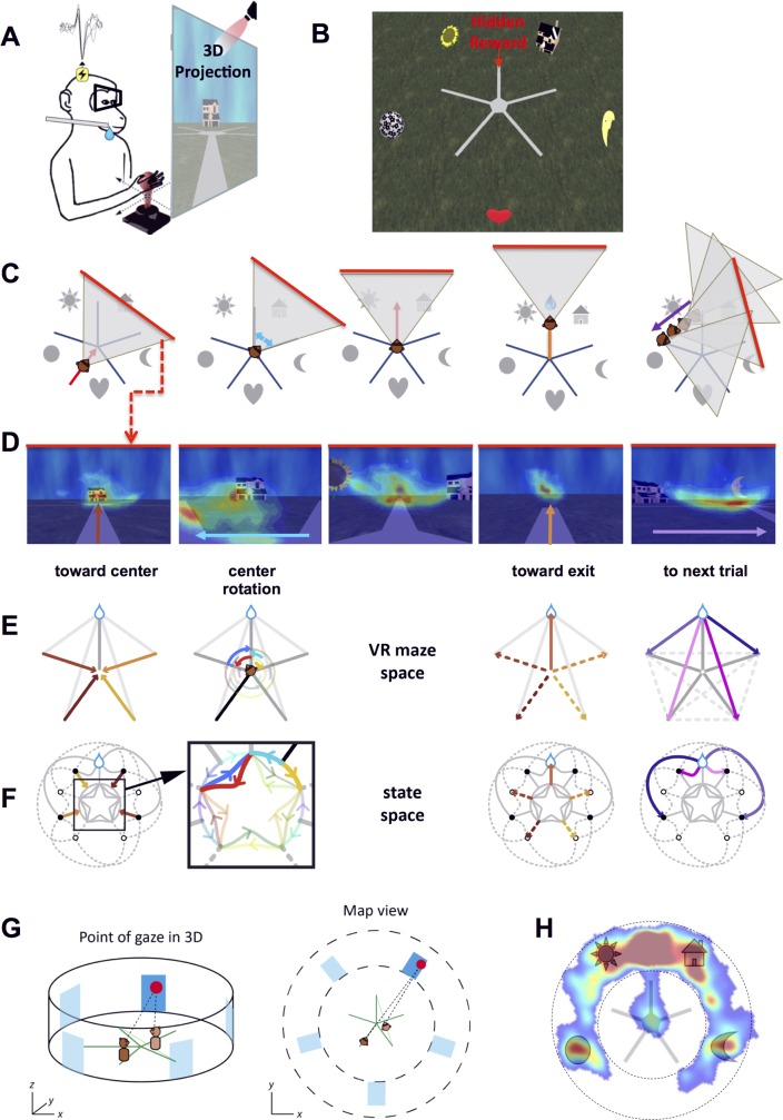
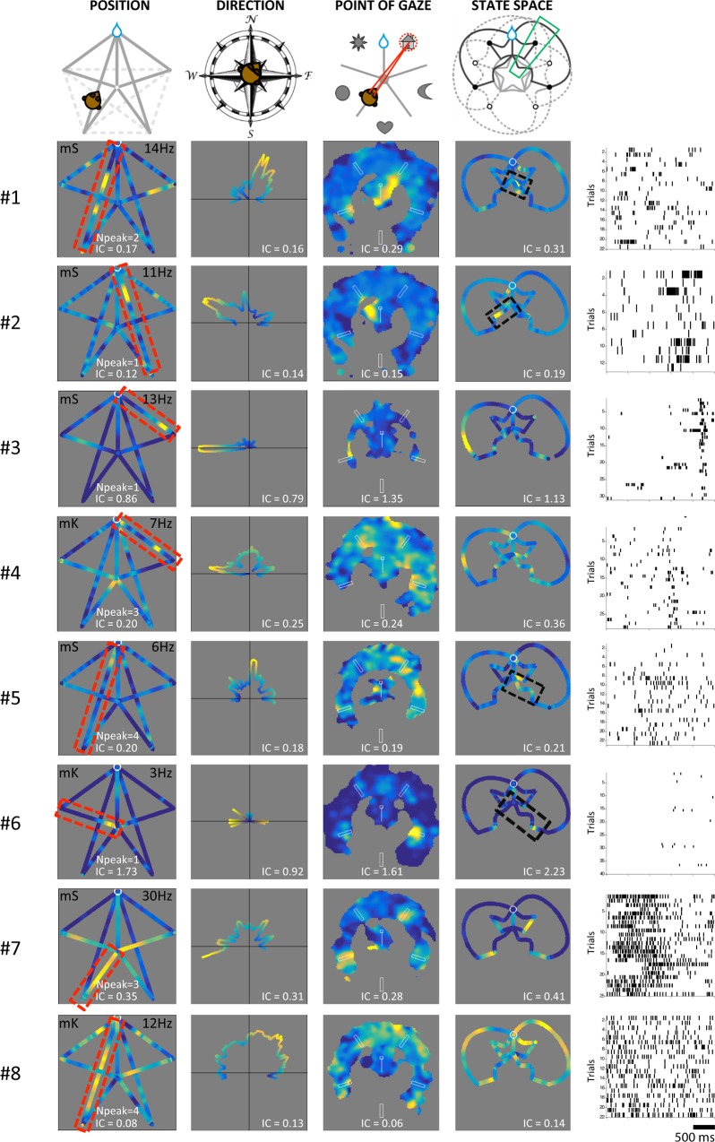
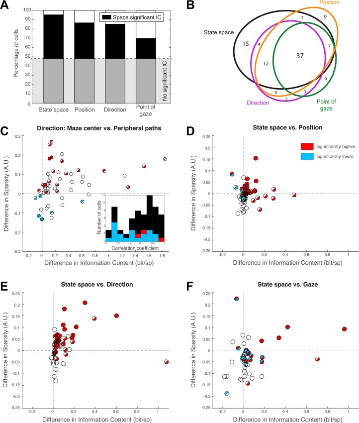
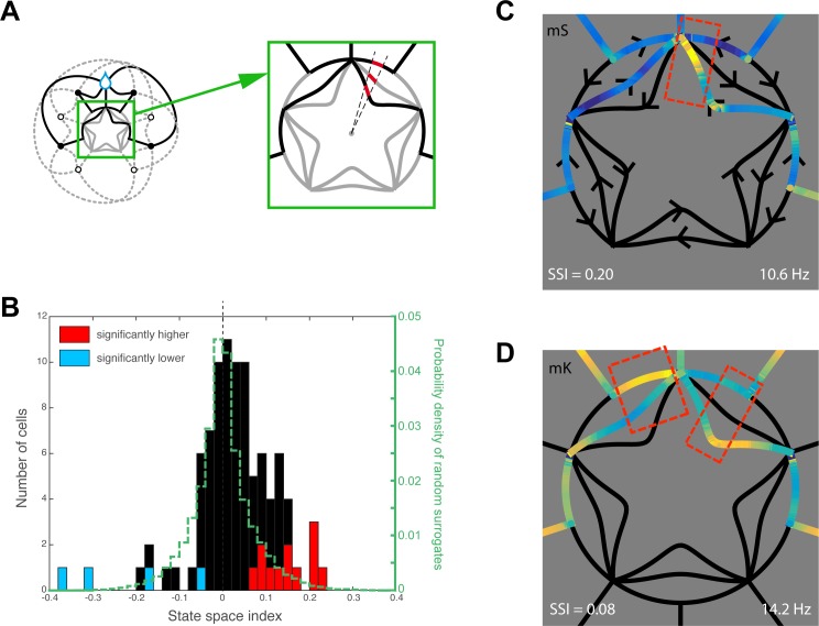
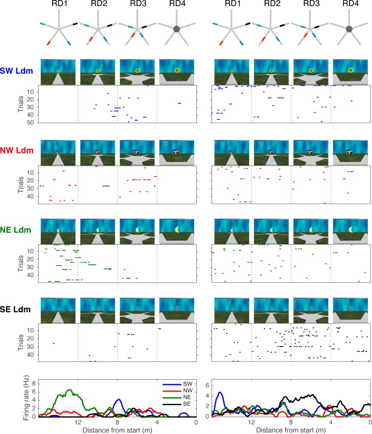
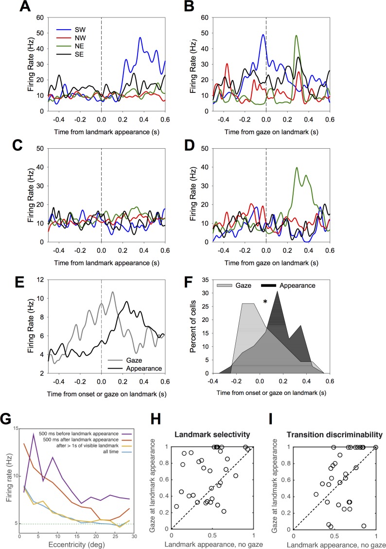
To elucidate how gaze informs the construction of mental space during wayfinding in visual species like primates, we jointly examined navigation behavior, visual exploration, and hippocampal activity as macaque monkeys searched a virtual reality maze for a reward. Cells sensitive to place also responded to one or more variables like head direction, point of gaze, or task context. Many cells fired at the sight (and in anticipation) of a single landmark in a viewpoint- or task-dependent manner, simultaneously encoding the animal's logical situation within a set of actions leading to the goal. Overall, hippocampal activity was best fit by a fine-grained state space comprising current position, view, and action contexts. Our findings indicate that counterparts of rodent place cells in primates embody multidimensional, task-situated knowledge pertaining to the target of gaze, therein supporting self-awareness in the construction of space.

Fig 1. Experimental setup and behavioral task.

A. Experimental setup. The animal was seated in front of a 152 x 114 cm screen on which a computer-generated scene was projected in stereo. The animal was equipped with shutter glasses synchronized with the projection and could move in the virtual world via a joystick. A juice dispenser delivered reward directly in the animal’s mouth when the monkey reached a hidden rewarded area. B. View from above of the star maze. Five landmarks were placed between the five arms of the maze at a radius twice the arms’ length. A reward was given to the animal when he reached the end of an arbitrarily chosen arm (in this case, the arm between the sunflower and the house). C. A sequential illustration of the animal’s position and field of view at key representative events of a trial. (1) The animal starts at one end of a path and moves towards the center, (2) turns left or right in the center, (3) chooses one path, (4) enters the chosen path and is rewarded at the end if correct, and (5) the animal is relocated (joystick disengaged) to the next start. D. First-person view of the five events described in C, with a heat map of the monkey’s gaze fixations overlaid on the scene illustrating the animal’s scanning interests. Arrows indicate the main direction of motion of the animal. E. Illustration of the steps described in C and D in the actual maze space. Monkey’s moves are represented by colored arrows. F. Illustration of the state space in which neuronal data was analyzed. The same steps as in E are plotted in the state-space graph with corresponding colors. For convenience, the animal’s current position in the graph also denotes the animal’s current straight ahead direction. For example, a position in the northeastern part of the graph corresponds to the animal viewing the northeast from its physical position. The state-space representation parses the animal’s trajectories into a series of action- or position-triggered transitions between choice points (graph vertices). Starting positions are figured as black dots. All actions that can eventually lead to the reward are in solid lines, while dashed lines indicate either erroneous actions leading to the end of unrewarded arms (open circles) or the path to the next start, outside the maze arms. This representation allows describing in a similar way the moves that include a translation and the purely rotational moves made in the center of the maze (expanded inset in the black square). Rotations of 72° (angle between two maze arms) are mapped to the central part of the graph, with counterclockwise rotations innermost (e.g., in red). Rotations of 36° (angle between landmark and maze arm) are mapped to the outer circular arcs (either clockwise or counterclockwise; e.g., in cyan). G. Mapping the animal’s 3-D point of regard. Left: three-dimensional schematic of the maze (green), monkey (brown), and point of gaze (red dot). Blue rectangles represent the location of the landmarks. For ease of representation, we define an invisible cylindrical wall running through the landmark centroids. Right: convention for the flattened representation of the point-of-gaze map. When directed further than the distance to the landmark wall, the point of gaze was computed as directed towards this wall; then, in a second step, this wall was flattened as an annulus to create the final 2-D map. H. Heat map of the point of gaze, overlaid on a schematic of the maze for one session (monkey S). The regions of interest explored by the animal are the ends of the paths, the landmarks, and the rewarded area.

Fig 2. Individual examples of cell activity in the four coding spaces studied.

Each space is mapped in a column (columns 1–4). The top row describes the structure of each of the coding spaces: monkey self-position (position), virtual head direction (direction), flattened gaze map (point of gaze), and state space (state space). Note that the state-space graph is drawn so that a sector like the one highlighted in green contains all the moves in which the monkey faces in the same direction (here, towards the northeastern landmark). Rows 2 to 9 represent the activity of eight individual cells that illustrate different firing patterns. The far-right column represents a raster histogram of the activity of each cell for all the laps that occurred in the path highlighted in red on the far-left figure for cells 3, 4, 7, and 8 or in black on the right adjacent figure for cells 1, 2, 5, and 6. In this raster representation, each row corresponds to an individual trial, and each tick represents an action potential, on a time window of 2.5 s. Monkey identity is indicated with mS or mK on the position maps. Underlying data can be found at http://dx.doi.org/10.6080/K0R49NQV.

Fig 3. Population statistics.

A. Proportion of responsive cells (cells with significant information content [IC], above gray line) and proportion of cells significantly coding each of the four spaces (black). Open bars correspond to cells with significant IC in another space. B. Representation of the main intersections amongst each subpopulation of cells represented in A. Most responsive cells carry significant activity in more than one coding space. C. Analysis of the responsive cells’ directional sensitivity and selectivity, comparing activity in the center of the maze to activity on peripheral paths to next start. The difference in information per spike is plotted against the difference in sparsity. Filled half-discs indicate significant differences, as established per cell (top-left half: significant sparsity difference; bottom-right half: significant information difference). Red indicates significantly positive differences (i.e., center > periphery), and blue indicates negative differences (center < periphery). Overall, the activity in the center is both more consistent and more direction specific. Inset: Distribution of the correlations between directional tuning in the center and in the periphery. Significantly high (red) and low (blue) correlations are indicated. D–F. Difference in information per spike versus difference in sparsity when comparing cell activity readout in state space to activity readout in position space (D), direction (E), and point of gaze (F). Same graphical conventions as in C. Statistical significance was obtained with permutation tests (surrogate spike datasets). Underlying data can be found at http://dx.doi.org/10.6080/K0R49NQV.

Fig 4. State-space selectivity.

A. Schematics illustrating the analysis method whereby activities corresponding to the same location (maze center) and direction (dashed sector) were compared on the different state-space transitions (in red). B. Histogram of the state-space selectivity indices across the responsive cells. Cells significantly invariant to current transition are in blue; cells significantly context-dependent are in red (permutation tests). The distribution of indices for the surrogate spike sets is shown in dashed green. C–D. State-space maps (restricted to the center) of two context-dependent cells. Underlying data can be found at http://dx.doi.org/10.6080/K0R49NQV.

Fig 5. Sensitivity to landmark identity and relative distance.

Left panel. Activity of a cell for each of the four landmarks viewed at four intervals of relative distances on the entry path (RD1 to RD4, see Materials and Methods). Top row: schema of the maze with these distance intervals illustrated as areas for each landmark (southwestern landmark in blue, northwestern in red, northeastern in green, and southeastern in black). The pictures above the rasters show a still image of the monkey’s view of the landmark at each relative distance symbolized by dotted lines on the raster (12, 8, 4), the last one being at 0. Each raster represents the activity of the cell to each landmark as the animal moves forward in the corresponding path. On these rasters, each line is a trial. The bottom graph shows the average cell activity over all trials. Right panel. Activity of a different cell recorded during the same session as the cell shown in the Left panel. Underlying data can be found at http://dx.doi.org/10.6080/K0R49NQV.

Fig 6. Landmark viewpoint-invariant versus viewpoint-dependent cells.

Top row: schematics of the monkey’s five different viewpoints for either the landmark immediately left or the landmark immediately right from the reward location. For every path, the landmark appears either on the animal’s left or right. A–C. Individual examples of cell activity (average and trial-by-trial raster histogram; cells numbered as in Fig 2) aligned on the landmark’s left or right entries in the animal’s field of view. The color codes correspond to the activity on the individual paths identified in the top row. Cells displayed in A and C discriminate between different viewpoints, while the cell displayed in B does not. D. Path selectivity index calculated for the different viewpoints of the landmark left or right of the reward (best landmark for each cell). In red are cells for which the index was significantly higher from chance (viewpoint dependent), and in blue are cells for which the index was significantly lower than chance (viewpoint invariant). The distribution of indices for the surrogate spike sets is shown in dashed green. Underlying data can be found at http://dx.doi.org/10.6080/K0R49NQV.

Fig 7. Modulation of cell selectivity by the point of gaze.

A. Mean activity of an example cell towards each of the four landmarks aligned on the entry of the landmark in the field of view or B aligned on the animal’s saccade towards the landmark. This cell has a preference for the southwestern landmark, and its activity peaks at the time of the saccade on the landmark. C–D. A second example cell with the same conventions as in A–B. This cell shows a higher activity to the southeastern landmark when the animal gazes at it (D) compared to when it enters the visual field (C). Those two examples illustrate two patterns of activity: (1) the activity of the cells peaks around the moment that the eyes reach the landmark, and (2) the gaze increases the firing rates associated with one landmark. E. The temporal dynamics of the mean cell activity with respect to landmark appearance or gaze on the landmark. F. Distribution of the latencies with respect to landmark appearance or foveation. G. Mean cell activity as a function of landmark eccentricity on the retina, considering four set of epochs relative to landmark appearance (see main text). Firing was always modulated by foveation but more so when the landmark recently appeared (red). Cells fired in anticipation of the landmark (purple), but activity was higher if the monkey had previously made a saccade close to its expected point of appearance. Dashed line: average firing rate. Note that the vertical scale does not begin at zero. H. Landmark selectivity indices calculated for activity aligned on landmark appearance when gaze was not directed to them versus activity aligned on landmark foveation following its appearance. I. Same as H for the path selectivity index. Underlying data can be found at http://dx.doi.org/10.6080/K0R49NQV.

References

1. O’Keefe J, Dostrovsky J. The hippocampus as a spatial map. Preliminary evidence from unit activity in the freely-moving rat. Brain Res. 1971;34: 171–175. - PubMed
1. Ahmed OJ, Mehta MR. The hippocampal rate code: anatomy, physiology and theory. Trends Neurosci. 2009;32: 329–338. 10.1016/j.tins.2009.01.009 - DOI - PMC - PubMed
1. Ravassard P, Kees A, Willers B, Ho D, Aharoni D, Cushman J, et al. Multisensory control of hippocampal spatiotemporal selectivity. Science. 2013;340: 1342–1346. 10.1126/science.1232655 - DOI - PMC - PubMed
1. Chen G, King JA, Burgess N, O’Keefe J. How vision and movement combine in the hippocampal place code. Proc Natl Acad Sci USA. 2013;110: 378–383. 10.1073/pnas.1215834110 - DOI - PMC - PubMed
1. Aronov D, Tank DW. Engagement of neural circuits underlying 2D spatial navigation in a rodent virtual reality system. Neuron. 2014;84: 442–456. 10.1016/j.neuron.2014.08.042 - DOI - PMC - PubMed
Publication types
LinkOut - more resources