Normalization and microbial differential abundance strategies depend upon data characteristics

Abstract

Background: Data from 16S ribosomal RNA (rRNA) amplicon sequencing present challenges to ecological and statistical interpretation. In particular, library sizes often vary over several ranges of magnitude, and the data contains many zeros. Although we are typically interested in comparing relative abundance of taxa in the ecosystem of two or more groups, we can only measure the taxon relative abundance in specimens obtained from the ecosystems. Because the comparison of taxon relative abundance in the specimen is not equivalent to the comparison of taxon relative abundance in the ecosystems, this presents a special challenge. Second, because the relative abundance of taxa in the specimen (as well as in the ecosystem) sum to 1, these are compositional data. Because the compositional data are constrained by the simplex (sum to 1) and are not unconstrained in the Euclidean space, many standard methods of analysis are not applicable. Here, we evaluate how these challenges impact the performance of existing normalization methods and differential abundance analyses.

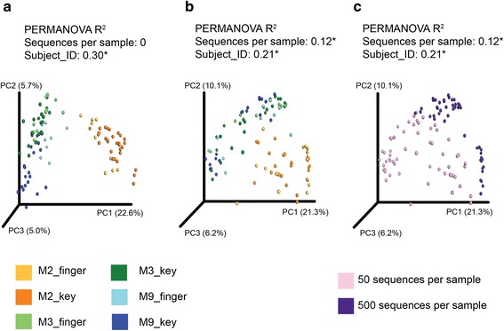
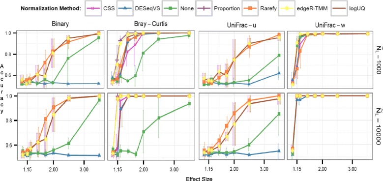
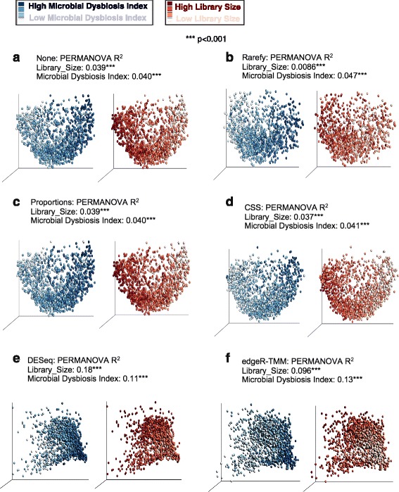
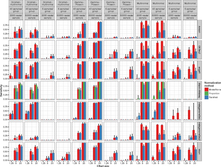
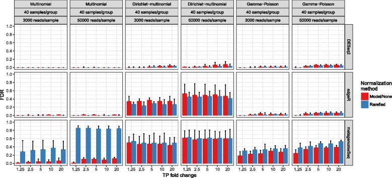
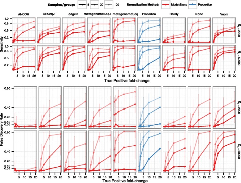
Results: Effects on normalization: Most normalization methods enable successful clustering of samples according to biological origin when the groups differ substantially in their overall microbial composition. Rarefying more clearly clusters samples according to biological origin than other normalization techniques do for ordination metrics based on presence or absence. Alternate normalization measures are potentially vulnerable to artifacts due to library size. Effects on differential abundance testing: We build on a previous work to evaluate seven proposed statistical methods using rarefied as well as raw data. Our simulation studies suggest that the false discovery rates of many differential abundance-testing methods are not increased by rarefying itself, although of course rarefying results in a loss of sensitivity due to elimination of a portion of available data. For groups with large (~10×) differences in the average library size, rarefying lowers the false discovery rate. DESeq2, without addition of a constant, increased sensitivity on smaller datasets (<20 samples per group) but tends towards a higher false discovery rate with more samples, very uneven (~10×) library sizes, and/or compositional effects. For drawing inferences regarding taxon abundance in the ecosystem, analysis of composition of microbiomes (ANCOM) is not only very sensitive (for >20 samples per group) but also critically the only method tested that has a good control of false discovery rate.

Conclusions: These findings guide which normalization and differential abundance techniques to use based on the data characteristics of a given study.

Keywords: Differential abundance; Microbiome; Normalization; Statistics.

Fig. 1

Normalization is critical to result interpretation. a The forensic study matching subject’s fingers to the keyboards they touched (Fierer et al.), rarefied at 500 sequences per sample. b, c Data not normalized, with a random half of the samples subsampled to 500 sequences per sample and the other half to 50 sequences per sample. b Colored by subject_ID. c Colored by sequences per sample. Nonparametric ANOVA (PERMANOVA) R ² roughly represents the percent variance that can be explained by the given variable. Asterisk (*) indicates significance at p < 0.01. The distance metric of unweighted UniFrac was used for all panels

Fig. 2

Comparison of common distance metrics and normalization methods across library sizes. Clustering accuracy, or fraction of samples correctly clustered, is shown for all combinations of four common distance metrics (panels arranged from left to right) across two library depths (panels arranged from top to bottom; N_L, median library size), six sample normalization methods (series within each panel), and several effect sizes (x-axis within panels). For all methods, samples below the 15th percentile of library size were dropped from the analysis to isolate the effects of rarefying. The x-axis (effect size) within each panel represents the multinomial mixing proportions of the two sample classes Ocean and Feces. A higher effect size represents an easier clustering task

Fig. 3

For unweighted distance measures, rarefying diminishes the effect of original library size. Nonparametric multivariate ANOVA (PERMANOVA) was calculated on the Inflammatory Bowel Disease (IBD) dataset of Gevers et al., using type I sequential sums of squares in the linear model (y~Library_Size + Microbial_Dysbiosis_Index). Unweighted UniFrac was used for clustering, except for letters (e–f) corresponding to weighted UniFrac DESeq and edgeR. The unweighted UniFrac distance matrix for DESeq and edgeR was zero, so a PCoA plot could not be made. For each letter (a–f), the left PCoA plot is colored according to microbial dysbiosis (left legend), and the right PCoA plot is colored according to library size (right legend)

Fig. 4

Differential abundance detection sensitivity with varied library sizes, that are approximately even on average between groups. Multinomial, Dirichlet-multinomial, and gamma-Poisson parameters were fit using actual OTU tables from many global environments. Fold change represents the fold change of the true positive OTUs from one condition (e.g., case) to another (e.g., control). The height of each bar represents the median value from three simulations. Vertical lines extend to the upper quartile of the simulation results. Model/none represents data analyzed with a parametric statistical model (e.g., DESeq) or no normalization. Blue lines in, e.g., the DESeq row represents the data that was rarefied, then DESeq was applied. Since the fitZIG model depends upon original library size information, the model has high FDR on rarefied data. A 0.01 pseudocount for edgeR was necessary to avoid log(0)

Fig. 5

Differential abundance detection false discovery rate with varied library sizes that are approximately even on average between groups. For simplicity, only those methods where the FDR exceeds or is close to 0.05 are shown. Full methods are in Additional file 7: Figure S6. Labels are the same as in Fig. 4

Fig. 6

Differential abundance detection performance when sample relative abundances do not reflect ecosystem relative abundances. 10% of OTUs are differentially abundant. For simplicity, only a multinomial model of 2000 OTUs was used, but is the same model as that in Figs. 4 and 5. Labels are the same as in Fig. 4

Fig. 7

False discovery rate increases when methods are challenged with very uneven library sizes. Real data from one body site was randomly divided into two groups, creating a situation in which there should be no true positives. a Uneven library sizes, 3 samples per group. b Uneven library sizes, 100 samples per group. For uneven library sizes, the group means differed by 10× (e.g., 40,000 sequences per sample vs. 4000 sequences per sample). The 45-degree line shows where the nominal FDR should equal the observed FDR. c Cumulative distribution functions of the effect sizes for 3, 20, and 100 samples per group presented in a and b. Voom was excluded because it was found to have a higher type I error rate than fitZIG

Fig. 8

On real datasets, methods disagree especially for few samples per group. FDR p < 0.05. Darker colors indicate a larger proportion of OTUs discovered by a technique or combination of techniques

References

1. Qin J, Li R, Raes J, Arumugam M, Burgdorf KS, Manichanh C, et al. A human gut microbial gene catalogue established by metagenomic sequencing. Nature. 2010;464(7285):59–65. doi: 10.1038/nature08821. - DOI - PMC - PubMed
1. Rodriguez RL, Konstantinidis KT. Estimating coverage in metagenomic data sets and why it matters. ISME J. 2014;8(11):2349–2351. doi: 10.1038/ismej.2014.76. - DOI - PMC - PubMed
1. Lozupone C, Lladser ME, Knights D, Stombaugh J, Knight R. UniFrac: an effective distance metric for microbial community comparison. ISME J. 2011;5(2):169–172. doi: 10.1038/ismej.2010.133. - DOI - PMC - PubMed
1. Paulson JN, Stine OC, Bravo HC, Pop M. Differential abundance analysis for microbial marker-gene surveys. Nat Methods. 2013;10(12):1200–1202. doi: 10.1038/nmeth.2658. - DOI - PMC - PubMed
1. Aitchison J. The statistical analysis of compositional data. J Roy Stat Soc B Met. 1982;44(2):139–177.
Publication types