Molecular Population Genetics

Abstract

Molecular population genetics aims to explain genetic variation and molecular evolution from population genetics principles. The field was born 50 years ago with the first measures of genetic variation in allozyme loci, continued with the nucleotide sequencing era, and is currently in the era of population genomics. During this period, molecular population genetics has been revolutionized by progress in data acquisition and theoretical developments. The conceptual elegance of the neutral theory of molecular evolution or the footprint carved by natural selection on the patterns of genetic variation are two examples of the vast number of inspiring findings of population genetics research. Since the inception of the field, Drosophila has been the prominent model species: molecular variation in populations was first described in Drosophila and most of the population genetics hypotheses were tested in Drosophila species. In this review, we describe the main concepts, methods, and landmarks of molecular population genetics, using the Drosophila model as a reference. We describe the different genetic data sets made available by advances in molecular technologies, and the theoretical developments fostered by these data. Finally, we review the results and new insights provided by the population genomics approach, and conclude by enumerating challenges and new lines of inquiry posed by increasingly large population scale sequence data.

Keywords: Drosophila; FlyBook; Hill–Robertson interference; distribution of fitness effects; genetic draft; linked selection; molecular population genetics; neutral theory; population genomics; population multi-omics.

Figure 1

Population genomics resources available for four Drosophila species. ● represents sequenced populations, and the size of the ● is proportional to the number of individuals sequenced. See an interactive and updateable version of this figure with additional information about each population at http://flybook-mpg.uab.cat. D. melanogaster populations: USTB, Tampa Bay, FL, n = 2; UST, Thomasville, GA, n = 2; USS, Selva, AL, n = 2; USB, Birmingham, AL, n = 2; USM, Meridian, MS, n = 2; USFL, Sebastian, FL, n = 2; BF, Freeport, Bahamas, n = 2; BGT, George Town, Bahamas, n = 2; BBH, Bullocks Harbor, Bahamas, n = 2; SS, Cockburn Town, San Salvador, n = 2; BM, Mayaguana, Bahamas, n = 2; B, Beijing, China, n = 15; CK, Kisangani, Congo, n = 2; CO, Oku, Cameroon, n = 13; EA, Gambella, Ethiopia, n = 24; EB, Bonga, Ethiopia, n = 5; ED, Dodola, Ethiopia, n = 8; EF, Fiche, Ethiopia, n = 69; EG, Cairo, Egypt, n = 32; EM, Masha, Ethiopia, n = 3; ER, Debre Birhan, Ethiopia, n = 5; EZ, Ziway, Ethiopia, n = 5; FRL, Lyon, France, n = 96; FRM, Montpellier, France, n = 20; GA, Franceville, Gabon, n = 10; AGA, Athens, GA, n = 15; GH, Accra, Ghana, n = 15; GU, Dondé, Guinea, n = 7; H, Port Au Prince, Haiti, n = 2; I, Ithaca, NY, n = 19; KM, Malindi, Kenya, n = 4; KN, Nyahururu, Kenya, n = 6; KO, Molo, Kenya, n = 4; KR, Marigat, Kenya, n = 6; KT, Thika, Kenya, n = 2; N, Houten, Netherlands, n = 19; NG, Maiduguri, Nigeria, n = 6; RAL, n = 205; RC, Cyangugu, Rwanda, n = 2; RG, Gikongoro, Rwanda, n = 27; SB, Barkly East, South Africa, n = 5; SD, Dullstroom, South Africa, n = 81; SE, Port Edward, South Africa, n = 3; SF, Fouriesburg, South Africa, n = 5; SP, Phalaborwa, South Africa, n = 37; T, Sorell, Tasmania, Australia, n = 18; TZ, Uyole, Tanzania, n = 3; UG, Namulonge, Uganda, n = 6; UK, Kisoro, Uganda, n = 5; UM, Masindi, Uganda, n = 3; W, Winters, CA, n = 35; ZH, Harare, Zimbabwe, n = 4; ZI, Siavonga, Zambia, n = 197; ZK, Lake Kariba, Zimbabwe, n = 3; ZL, Livingstone, Zambia, n = 1; ZO, Solwezi, Zambia, n = 2; ZS, Sengwa, Zimbabwe, n = 5; ZW, Victoria Falls, Zimbabwe, n = 9; MAD, Tampa Bay, FL, n = 2; NAIS, Thomasville, GA, n = 2; WIN, Selva AL, n = 2; NOU, Birmingham, AL, n = 2; NAN, Meridian, MS, n = 2. D. simulans populations: MAD, Madagascar, n = 12; NAIS, Nairobi, Kenya, n = 10; WIN, Winters, CA, n = 2; NOU, Noumea, New Caledonia, n = 1; NAN, Nanyuki, Kenya, n = 1. D. yakuba populations: NAIY, Nairobi, Kenya, n = 10; NGU, Nguti, Cameroon, n = 10; TAI, Taï Rainforest, Liberia, n = 1. D. mauritiana populations: MAU, Mauritius, n = 117.

Kimura’s neutral theory of molecular evolution. By postulating the revolutionary new concept of neutral variants, Kimura’s neutral theory summarizes molecular evolution in one the most elegant mathematical expressions in science. The expression $K={\mu }_0$ (the rate of molecular evolution equals the neutral mutation rate) unifies the three levels of genetic variation from its origin to its substitution in the population: mutation (individual level), polymorphism (population level), and divergence (species level). According to the neutral theory, intrapopulation polymorphism is just a random walk of variants in their process to fixation or loss (represented for species A: gray, neutral mutations; maroon, strongly deleterious mutations; see also Figure 3B). Orange arrows represent the average lifetime of a neutral mutation from its appearance to its fixation in the population (1/μ₀).

Figure 2

DFE according to the (nearly) neutral theory of molecular evolution. (A) In the 1960s, according to the Kimura’s neutral theory. (B) In the 1970s, after the extension of the neutral theory by Ohta. Different selection coefficients of mutations are colored in a gradient from maroon (strongly deleterious), red (slightly deleterious), gray (neutral), light green (slightly advantageous), and dark green (advantageous).

Figure 3

Molecular evolutionary rate (K) as a function of (A) the DFE, (B) the probability of fixation of new mutations entering the population, and (C) the rate at which new mutations enter the population per site per generation (see text for details). Different selection coefficients of mutations are colored in a gradient from maroon (strongly deleterious), red (slightly deleterious), gray (neutral), light green (slightly advantageous), and dark green (advantageous).

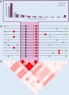
Signatures of a selective sweep in the genome (A) A reduction in genetic diversity, (B) a skew toward rare derived alleles, and (C) an increase in LD (see text for details). Colored ● reflects different classes of mutations according to their fitness effects: maroon, strongly deleterious (very infrequent, in their way to elimination by natural selection); red, slightly deleterious; gray, neutral; light green, slightly advantageous; dark green, advantageous. Note that in the region of the selective sweep (purple), an advantageous mutation has been driven to fixation together with its linked neutral and nearly neutral variants. In this region, genetic diversity is reduced, most polymorphisms are shared among different chromosomes (high LD), while recently arisen mutations are still at low frequency (gray ● present in two chromosomes).

Figure 4

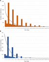
The footprint of deleterious selection on indel variation. Indel size distribution of (A) deletions and (B) insertions in coding regions (bars) and short introns (for comparison, gray line). The size distribution of indels in coding regions has discrete peaks for indel sizes in multiples of 3 bp. This remarkable pattern is a classroom example of the footprint that natural selection against frameshifting indels leaves, compared to a more relaxed selection for insertions and deletions spanning complete codons or short introns. Data from Massouras et al. (2012) and Huang et al. (2014).

Figure 5

Representation of the cost of linkage on selected sites, or HRi. Arrows indicate adaptive (green) and deleterious (red) mutations, while their length indicates the intensity of selection. (A) When two or more adaptive mutations occur in separate haplotypes without recombination (left), only one of them can be fixed in the population and thus mutations compete for their fixation. However, when recombination is sufficiently high (right), the two haplotypes can exchange alleles and generate a new haplotype that carries both adaptive mutations and can be fixed. (B) In the presence of both adaptive and deleterious mutations without recombination (left), all alleles compete; as a result, deleterious alleles may be dragged to fixation if the intensity of selection favoring a nearby adaptive mutation is high, or adaptive alleles may be lost if the joint strength of negative selection is higher. With recombination (right), deleterious alleles can be removed and adaptive alleles can be fixed without interfering with each other. Adapted from Barrón (2015).

Figure 6

Relationship between recombination and adaptation in the D. melanogaster genome. The adaptation rate of a genomic region increases with the recombination rate until a threshold value of recombination (∼2 cM/Mb) in which adaptation rate reaches an asymptote. The shaded area represents the reduction of adaptive rate due to the cost of genome linkage, whose value has been estimated for the first time at ∼27% in a North American population of D. melanogaster. r_opt is the optimal baseline value of recombination above which any detectable HRi vanishes (see text for details). Adaptation index: K_a+, rate of adaptive nonsynonymous substitution. Negative values mean fixation of deleterious mutations. Data from Castellano et al. (2016).

References

1. 1000 Genomes Project Consortium , 2012. An integrated map of genetic variation from 1,092 human genomes. Nature 491: 56–65. - PMC - PubMed
1. 1000 Genomes Project Consortium , 2015. A global reference for human genetic variation. Nature 526: 68–74. - PMC - PubMed
1. 1001 Genomes Consortium , 2016. 1,135 genomes reveal the global pattern of polymorphism in Arabidopsis thaliana. Cell 166: 481–491. - PMC - PubMed
1. Achaz G., 2009. Frequency spectrum neutrality tests: one for all and all for one. Genetics 183: 249–258. - PMC - PubMed
1. Adams M. D., Celniker S. E., Holt R. A., Evans C. A., Gocayne J. D., et al. , 2000. The genome sequence of Drosophila melanogaster. Science 287: 2185–2195. - PubMed
LinkOut - more resources