Controllability and observability in complex networks - the effect of connection types

Abstract

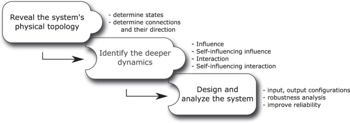
Network theory based controllability and observability analysis have become widely used techniques. We realized that most applications are not related to dynamical systems, and mainly the physical topologies of the systems are analysed without deeper considerations. Here, we draw attention to the importance of dynamics inside and between state variables by adding functional relationship defined edges to the original topology. The resulting networks differ from physical topologies of the systems and describe more accurately the dynamics of the conservation of mass, momentum and energy. We define the typical connection types and highlight how the reinterpreted topologies change the number of the necessary sensors and actuators in benchmark networks widely studied in the literature. Additionally, we offer a workflow for network science-based dynamical system analysis, and we also introduce a method for generating the minimum number of necessary actuator and sensor points in the system.

Figure 1

Representations of a state-transition matrix. (a) Illustrative state equation with four state variables. (b) Network representation of the dynamical system. (c) The adjacency matrix of the network is the transpose of the state-transition matrix.

Figure 2

Maximum matching in directed networks. (a) Simple, unweighted directed graph with four nodes and four edges. (b) Result of maximum matching in the directed network. Edge a ₂₁ cannot be a member of the disjoint set of edges, as it has a common starting point with a ₃₁ and a common end point with a ₂₃. End points of matched edges are matched nodes. (c) Undirected representation of the directed network. For each node in the directed network there are two nodes in the undirected representation, one for outgoing edges and one for incoming edges. The representation of edges is obvious. The result of maximum matching is the same in both directed and undirected representations.

Figure 3

Dynamics of two state variables. (a) Basic connection without additional edges represents the ‘logical’ or ‘structural’ relationship between the elements. (b) Source state variable influences itself as well, for example, it represents a variable that has a capacity which changes due to the connection. (c) The change of the terminating state variable also depend on its value, e.g. accumulation. (d) Combined dynamics of types (b,c). (e) The symmetric edge-pair shows that the influence is undirected, or the strength of the influence depends on the other state variable, as the signal flows in causal bond graphs. (f) Combined dynamics of types (b,e). (g) Combined dynamics of types (d,e).

Figure 4

Physical representation of water tanks. State variables represent water levels in the tanks. Flow rates F ₁ and F ₂ show how the water flows through the pipes from the first tank into the others.

Figure 5

Physical representation and state-transition matrix-based representation of water tanks. The difference between the physical structure and the structure of the properly modelled state-transition matrix is significant.

Figure 6

The examined four types of water-tank network models with associated inputs (u) and outputs (y). (a) Physical connection between state variables. (b) Self-influencing represents integrating node dynamics. (c) Interaction represents balanced dynamics (material balance). (d) Detailed model of the system. Already this small example clearly shows how connection types change the number and location of the driver and sensor nodes. The driver and sensor nodes were determined by the path-finding method introduced in section II of the Supplementary Information.

Figure 7

Determined flowchart for system design and analysis. Since connection types can be determined according to the topology of the systems, we strongly recommend following the proposed workflow and taking into account deeper dynamics to obtain more accurate and reliable results.

Figure 8

Initial percentage of self-influence and interactions in network sets. By examining real networks and dynamical systems, we get unequivocal results of structural differences. (a) Network Set I does not exhibit self-influence, and Network Set II does not exhibit them except in four cases, and only two of them exhibit more than 8% of self-influencing edges in their topologies. In contrast, more than 50% of self-influencing interactions in Network Set III are observed, i.e. more than half of the state variables influence themselves in dynamical systems. The median is almost 100%, so these dynamics are usual in dynamical systems. (b) In Network Set I usually less than 35% of interaction type edges are observed. In the case of Network Set II, results are a little higher. In Network Set III only four systems contain less than 100% of interactions, so in dynamical systems these dynamics is always present.

Figure 9

Proportion of driver and sensor nodes in networks with different connection types. Bar diagrams containing the mean of the proportion of driver (a) or sensor (b) nodes grouped according to network types. Apart from influence the numbers on the top of the bars show the reduction of driver and sensor nodes compared to the original.

Figure 10

Number of driver and sensor nodes as a function of the presence of self-influence and interactions. The heat map clearly shows that with the increase in self-influencing and interaction type edges the number of driver and sensor nodes decreased progressively. The white bars in heat maps of celegans network are caused by the initial existence of 9% of interaction type connections.

References

1. Liu Y-Y, Slotine J-J, Barabási A-L. Controllability of complex networks. Nature. 2011;473:167–173. doi: 10.1038/nature10011. - DOI - PubMed
1. Liu Y-Y, Slotine J-J, Barabási A-L. Observability of complex systems. Proceedings of the National Academy of Sciences. 2013;110:2460–2465. doi: 10.1073/pnas.1215508110. - DOI - PMC - PubMed
1. Yan G, et al. Spectrum of controlling and observing complex networks. Nature Physics. 2015;11:779–786. doi: 10.1038/nphys3422. - DOI
1. Ruths J, Ruths D. Control profiles of complex networks. Science. 2014;343:1373–1376. doi: 10.1126/science.1242063. - DOI - PubMed
1. Pósfai, M., Liu, Y.-Y., Slotine, J.-J. & Barabási, A.-L. Effect of correlations on network controllability. Scientific Reports3 (2013). - PMC - PubMed
Publication types
LinkOut - more resources