. 2017 Jan 18;4(1):160741.
doi: 10.1098/rsos.160741. eCollection 2017 Jan.

Detecting and characterizing high-frequency oscillations in epilepsy: a case study of big data analysis

Affiliations

Detecting and characterizing high-frequency oscillations in epilepsy: a case study of big data analysis

Liang Huang et al. R Soc Open Sci. .

Abstract

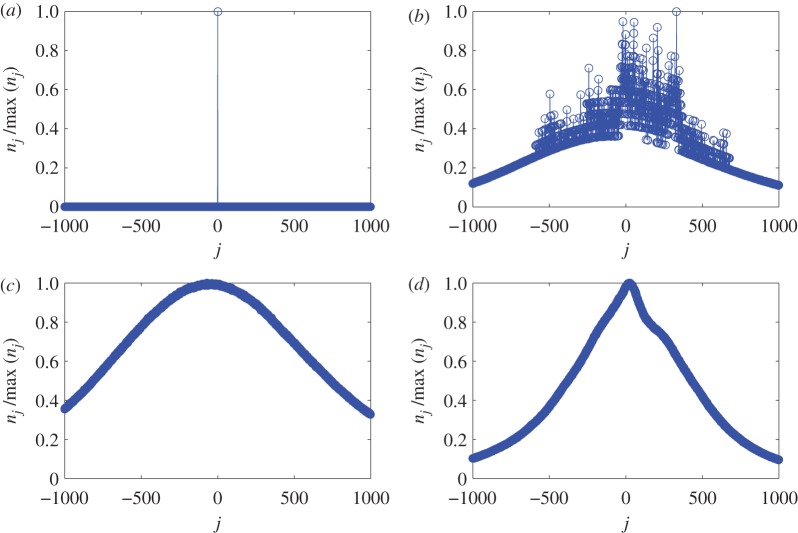
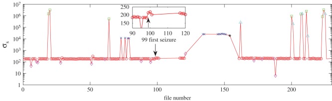
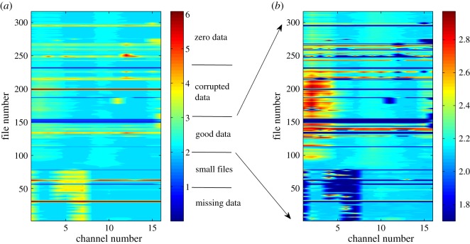
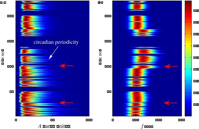
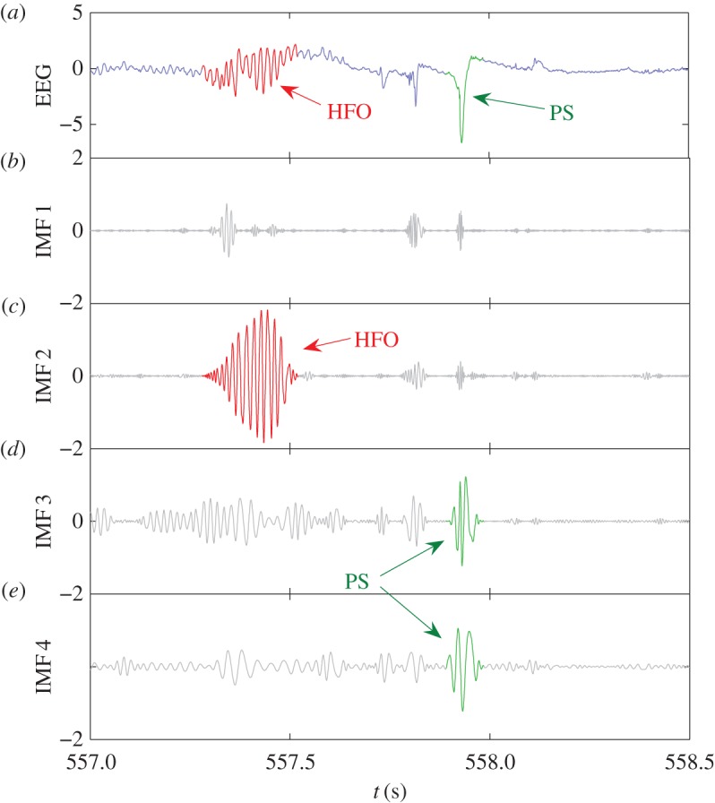
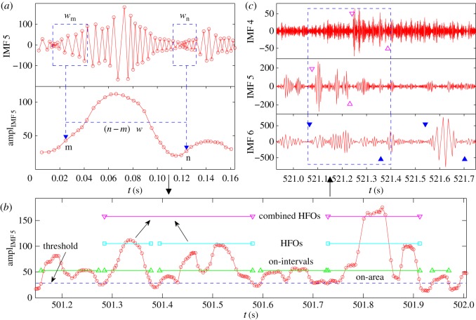
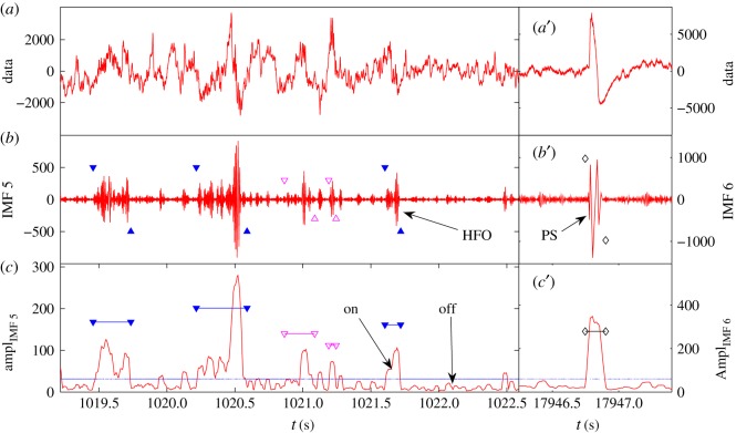
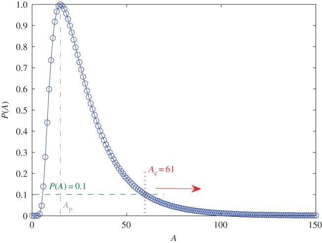
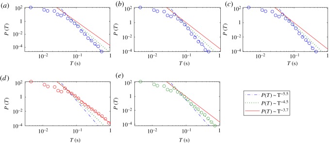
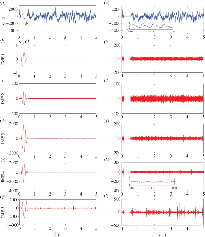
We develop a framework to uncover and analyse dynamical anomalies from massive, nonlinear and non-stationary time series data. The framework consists of three steps: preprocessing of massive datasets to eliminate erroneous data segments, application of the empirical mode decomposition and Hilbert transform paradigm to obtain the fundamental components embedded in the time series at distinct time scales, and statistical/scaling analysis of the components. As a case study, we apply our framework to detecting and characterizing high-frequency oscillations (HFOs) from a big database of rat electroencephalogram recordings. We find a striking phenomenon: HFOs exhibit on-off intermittency that can be quantified by algebraic scaling laws. Our framework can be generalized to big data-related problems in other fields such as large-scale sensor data and seismic data analysis.

Keywords: big data analysis; electroencephalogram; empirical modedecomposition; epileptic seizures; high-frequency oscillations; nonlinear dynamics.


Figures

Figure 1.
Figure 1.
Pretreatment of massive data from rat EEG. Different types of distributions of nj for Rat004 channel 02. For each panel, the y-axis is normalized by the maximum of nj. The four panels correspond to: (a) a corrupted file with a large number of zeros (file no. 20), (b) a bad recording with repetitions of oscillating patterns (file no. 73), (c) a normal file without transitions (file no. 77) and (d) a file containing a seizure (file no. 99).
Figure 2.
Figure 2.
Statistical properties of massive data from rat EEG. Standard deviation σs for Rat004 channel 02. Red circles denote the normal files; green squares are the files with large numbers of zeros; blue crosses are corrupted files; pink diamonds are small files; cyan triangles are small files with many zeros; black star is small corrupted files. The arrow marks the file 99 which has the first seizure. The inset shows the enlarged area around file 99 on a linear scale.
Figure 3.
Figure 3.
Contour representation of massive data from rat EEG. Contour plot of log10σs for Rat001. (a) The whole σs range. Different types of data are classified according to the value of log10σs. In (b), the contour is for values of 102σs103 (good data), and the remaining values of σs are set to 50 so that the dark blue area marks all abnormal data.
Figure 4.
Figure 4.
Typical EMD representation of massive rate EEG data. (a) Contour plot of normalized distribution of amplitude A (in arbitrary units) varying in time of a particular EMD mode of interest (IMF5, approx. 200 Hz) for channel 11 in CA1 of EEG recording of a rat over a two-month period. The all-blue region indicates corrupted files. Each file is a 7 h recording at the sampling frequency 12 kHz. Thus, the vertical axis ‘file no.’ indicates time. The distribution is calculated and then normalized by the maximum value for each file. The rat underwent surgery between file 28 and file 29, and the first seizure occurred in file 99, as indicated by the red arrows. The comb-like structure indicates the circadian periodicity. (b) Normalized distribution of the frequency f of the mode.
Figure 5.
Figure 5.
Example of EMD-based HFO detection from EEG data. (a) A 1.5 s segment of normalized EEG data containing an HFO and a population spike. (be) The IMFs in the frequency range of interest. The HFO is revealed in IMF 2 and the population spike is revealed in IMF 3 and IMF 4.
Figure 6.
Figure 6.
Illustration of HFO detection method. The method consists of three steps. (a) Computing the amplitude function from each IMF generated by EMD. The size of the moving window is w=7 periods (indicated by the blue dashed boxes). The time step for the moving window is Δw. (b) For each IMF, we locate the on-intervals, find HFOs, and combine adjacent HFOs if they are too close to each other. The blue dashed line is the threshold chosen for the segment of the amplitude function. (c) Classifying HFOs in terms of their frequencies, e.g. ripples (solid blue triangles), fast ripples (open magenta triangles) and then combining overlapping HFOs across different IMFs, as shown in the blue dashed box.
Figure 7.
Figure 7.
Example of successful HFO and PS detection. (a) Original EEG data plot of about 3 s. (b) IMF 5 plot with solid blue triangles marking the ripples and open magenta triangles marking the fast ripples. (c) The amplitude of IMF 5. The horizontal blue line is the threshold for separating on/off intervals of HFOs. The threshold is calculated from the amplitude data segment of about 1 h. The computational parameters are aμ=1 and aσ=1. (a)–(c) The original data, IMF 6, and its amplitude function, respectively. The black diamonds mark the position of the population spikes.
Figure 8.
Figure 8.
Determination of threshold Ac. Normalized distribution P(A) of the amplitude A for files 1–28 for the same mode as in figure 4, where Ap is the value of amplitude at the peak of the distribution. For example, by setting P(A)=0.1 and assuming that Ac>Ap, Ac can be determined to be 61. If P(A) takes a smaller value, then Ac will be larger.
Figure 9.
Figure 9.
Statistical and scaling behaviours of HFOs. Distributions of on-interval T of IMF 5 (channel 11, figure 4): (ae) for files 1–28, 29–51, 52–94, 100–172, 175–223, respectively. The numbers of on-intervals are 344 310, 314 698, 431 674, 498 947 and 510 096 for (ae), respectively. An algebraic distribution is observed with different exponents for different segments. The exponent for the solid, dotted and dash-dotted lines are 3.7,4.5 and 5.5, respectively. The threshold Ac is chosen such that P(Ac)=0.02 for all the segments.
Figure 10.
Figure 10.
Statistical and scaling behaviours of HFOs, more examples. Distributions of on-interval T of IMF 5 (channel 6 of rat 9): (af) for files 1–19, 32–57, 63–72, 78–97, 98–118 and 119–149, corresponding to the pre-stimulation state, post-stimulation state, evolving towards seizure, status epilepticus phase, epilepsy latent period and spontaneous/recurrent seizure period, respectively. The numbers of on-intervals are 354 499, 561 669, 300 291, 458 649, 293 118 and 438 919 for (af), respectively. An algebraic distribution is observed with different exponents for different segments, where the exponents are 5.7, 3.3, 2.9 for dash-dotted line, solid line and dotted line, respectively. The criterion for choosing the threshold Ac is the same as in figure 9.
Figure 11.
Figure 11.
A demonstration of adding small oscillations in EMD computation to eliminate spurious large values in IMFs. (a) A 5 s segment of data with about 0.4 s zeros, as indicated by the dotted circle. (bf) The first 5 IMFs directly calculated from the data in (a). (g) Data (a) with added small oscillations on the scale of unity (see text), which is almost invisible from the figure. (hl) The first 5 IMFs calculated from the data in (g). Insets of (g) and (k) show magnification of the zero region. Note that the scale of the y axis is much larger in (bf) than those in (hl). The anomalies appeared in (bf) are effectively removed by the simple method of adding small oscillations to the data segment.

Similar articles

Cited by

References

    1. Marx V. 2013. Biology: the big challenges of big data. Nature (London) 498, 255–260. (doi:10.1038/498255a) - DOI - PubMed
    1. Sagiroglu S, Sinanc D. 2013. Big data: a review. In 2013 Int. Conf. on Collaboration Technologies and Systems (CTS), San Diego, CA, pp. 42–47. IEEE.
    1. Katal A, Wazid M, Goudar RH. 2013. Big data: issues, challenges, tools and good practices. In Sixth Int. Conf. on Contemporary Computing (IC3), Noida, pp. 404–409. IEEE.
    1. Chen M, Mao SW, Zhang Y, Leung VCM. 2014. Big data related technologies, challenges and future prospects. Berlin, Germany: Springer.
    1. Fan JQ, Han F, Liu H. 2014. Challenges of big data analysis. Nat. Sci. Rev. 1, 293–314. (doi:10.1093/nsr/nwt032) - DOI - PMC - PubMed

LinkOut - more resources