Towards a comprehensive framework for movement and distortion correction of diffusion MR images: Within volume movement

Abstract

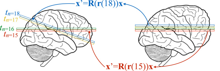
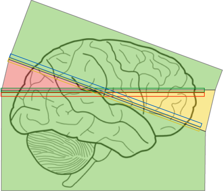
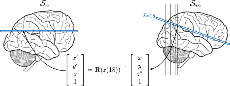
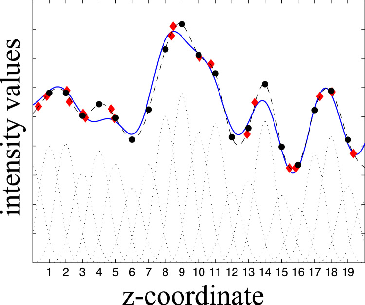
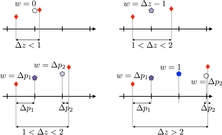
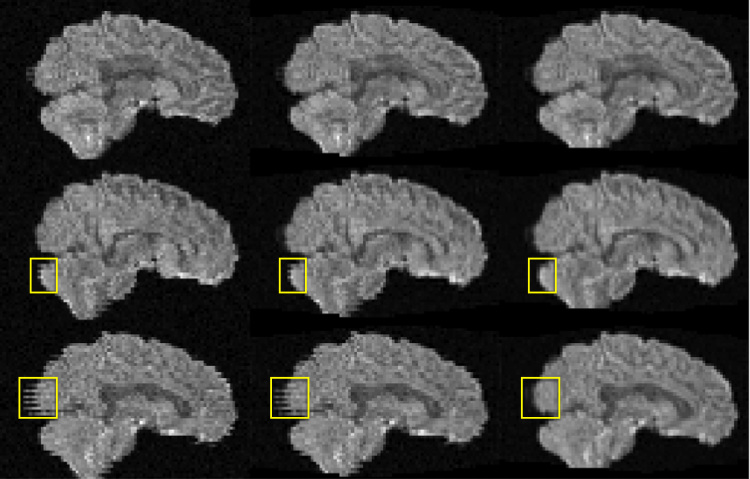
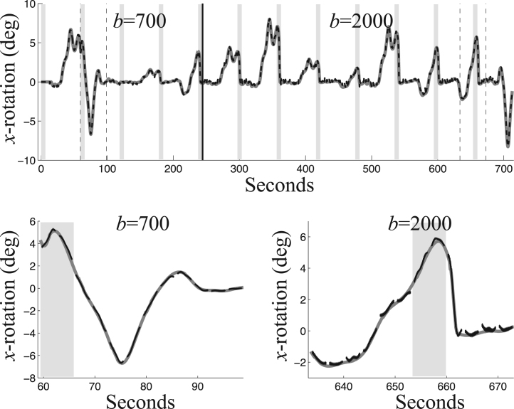
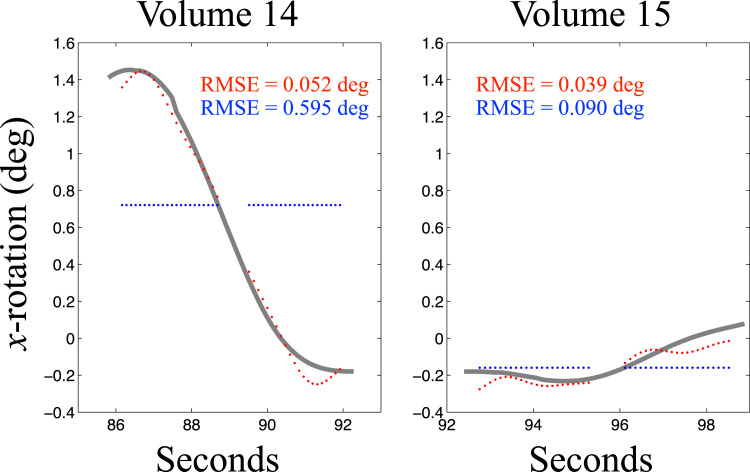
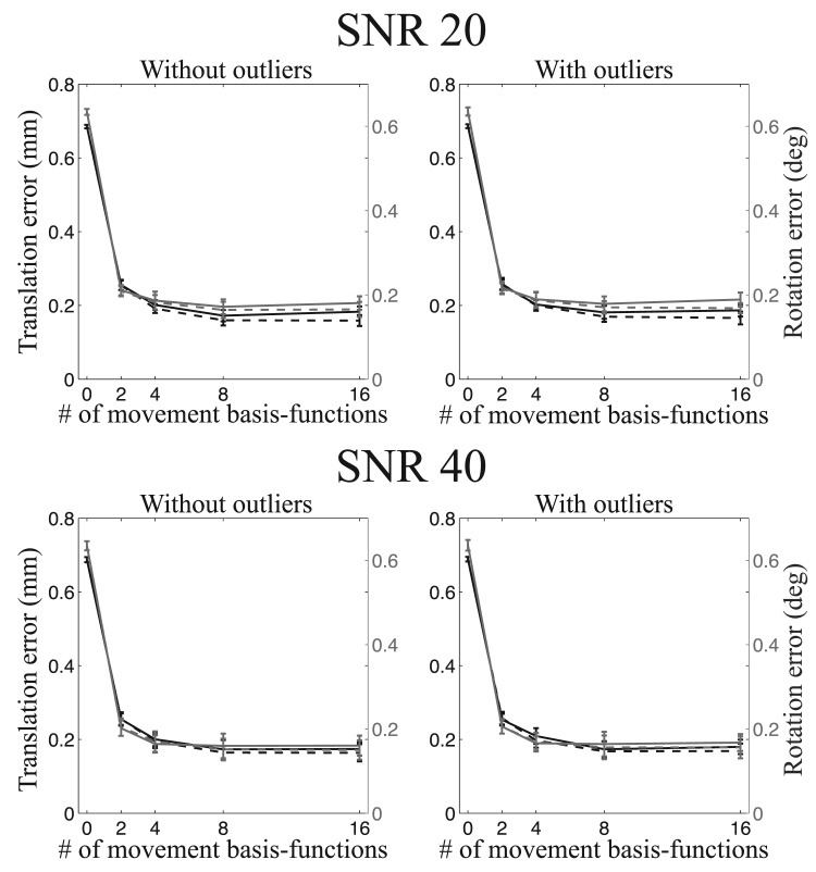
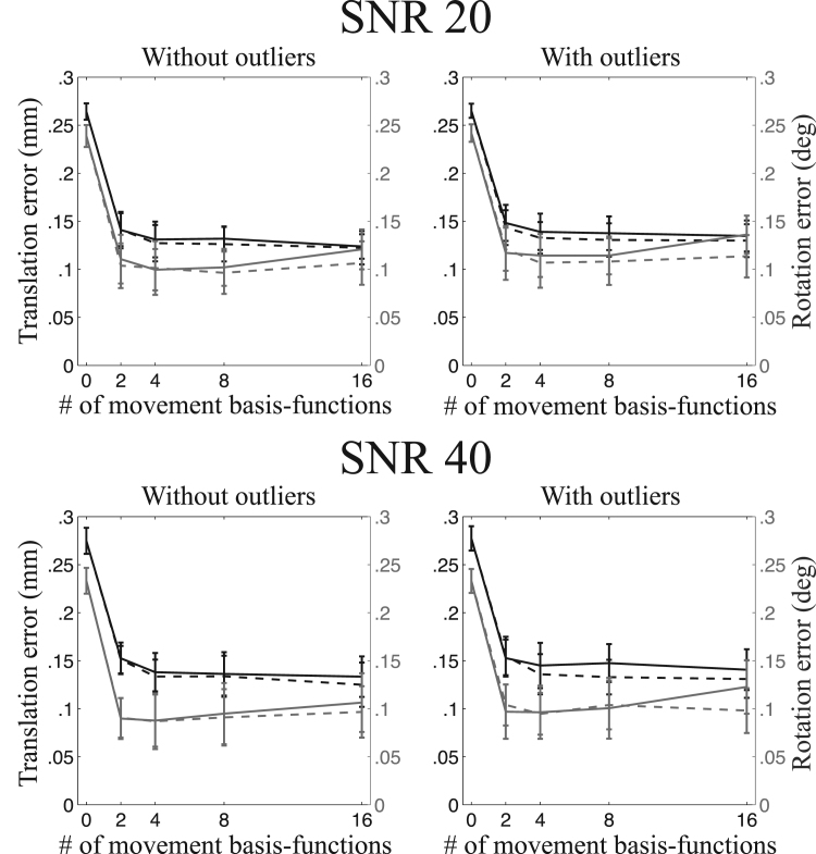
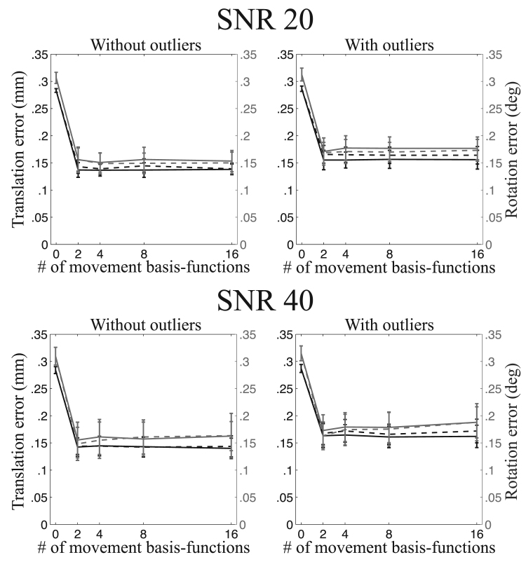
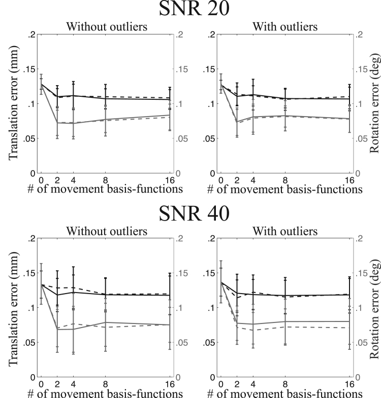
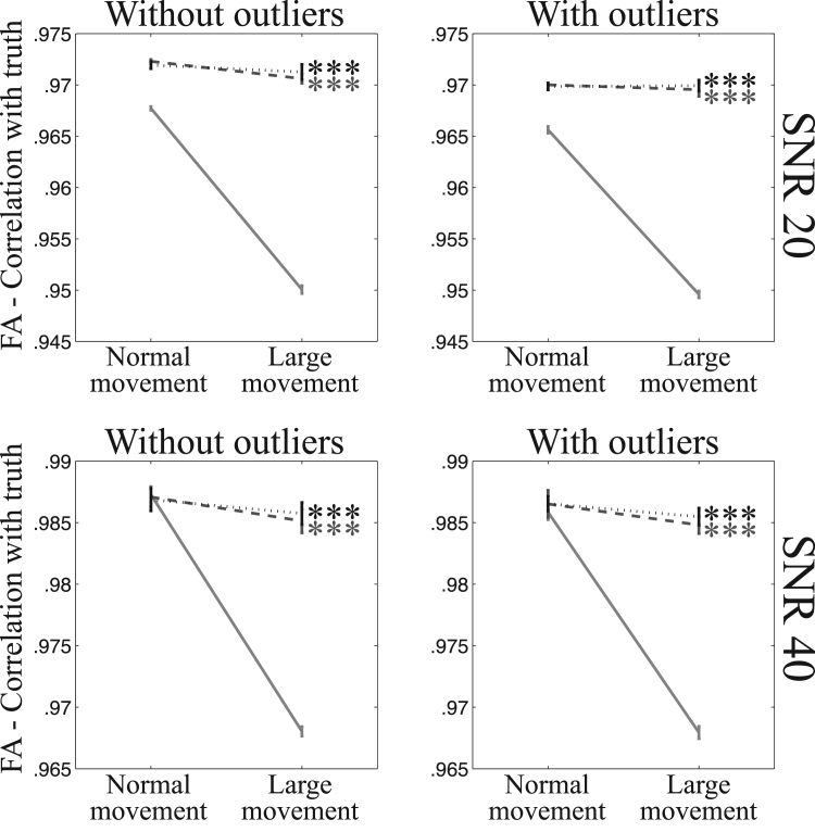
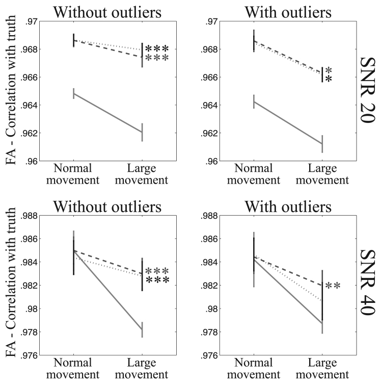
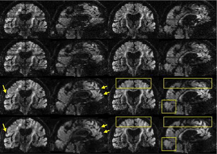
Most motion correction methods work by aligning a set of volumes together, or to a volume that represents a reference location. These are based on an implicit assumption that the subject remains motionless during the several seconds it takes to acquire all slices in a volume, and that any movement occurs in the brief moment between acquiring the last slice of one volume and the first slice of the next. This is clearly an approximation that can be more or less good depending on how long it takes to acquire one volume and in how rapidly the subject moves. In this paper we present a method that increases the temporal resolution of the motion correction by modelling movement as a piecewise continous function over time. This intra-volume movement correction is implemented within a previously presented framework that simultaneously estimates distortions, movement and movement-induced signal dropout. We validate the method on highly realistic simulated data containing all of these effects. It is demonstrated that we can estimate the true movement with high accuracy, and that scalar parameters derived from the data, such as fractional anisotropy, are estimated with greater fidelity when data has been corrected for intra-volume movement. Importantly, we also show that the difference in fidelity between data affected by different amounts of movement is much reduced when taking intra-volume movement into account. Additional validation was performed on data from a healthy volunteer scanned when lying still and when performing deliberate movements. We show an increased correspondence between the "still" and the "movement" data when the latter is corrected for intra-volume movement. Finally we demonstrate a big reduction in the telltale signs of intra-volume movement in data acquired on elderly subjects.

Keywords: Diffusion; Interpolation; Movement; Registration; Slice-to-volume.

Fig. 1

This figure serves the double purpose of explaining the intra-volume movement problem as well as our forward spatial model. To understand the problem, consider a sequential single-slice sequence where slices 15 and 16 have just been acquired, then the subjects move (“looking up into the sky”) so that slices 17 and 18 are acquired at the positions indicated in the schematic on the left. The reconstruction process does not know that the subject has moved and will stack the slices on top of each other as seen on the right hand side. If we assume that the subject stays in this new position for the remaining slices the apparent shape of the brain will now be as seen on the right (looking more like a sperm whale than a brain), as opposed to the true shape shown on the left. In order to understand the forward model, assume that all movement is known such that we can accurately calculate the matrices $\mathbf{R}(\mathbf{r}(15))$ and $\mathbf{R}(\mathbf{r}(18))$. The image ${\widehat{f}}_i$ from Eq. (1) serves as the image on the left, and is hence “known”. The aim of the forward model is now to calculate the image on the right given that we know $\mathbf{B}$, i.e. all the movements. This is performed using the following strategy: for all coordinates $\mathbf{x}$ on the right calculate $\mathbf{x}\prime$, map $\mathbf{x}\prime$ into the regular grid of ${\widehat{f}}_i$ and use standard spline interpolation to calculate an intensity ${\widehat{f}}_i(\mathbf{x}\prime )$ that is written into $f_i(\mathbf{x})$ on the right. Using this strategy it is possible to predict the “observed” image for any set of movements $\mathbf{B}$.

Fig. 2

This figure shows the same acquisition situation as Fig. 1. After acquisition of slices 15 (red slice) and 16 (green) the subject moved (“looked into the sky”) and slices 17 and 18 were acquired in the locations shown in yellow and blue respectively. We also assume that prior to slice 15 all slices were acquired with the subject in the same position and hence were parallel to slice 15 and correspondingly all slices after slice 18 were parallel to slice 18. The green parts of the volume have been acquired once, and once only, on a regular grid and standard interpolation would in principle be feasible. The yellow part has been acquired twice and there will be spots where voxel values from one slice will almost exactly coincide (spatially) with values from another slice and these values will have to be reconciled. Finally the red part has not been acquired at all which means that an interpolation will need to fill in values a long distance from the nearest observed values. For an interleaved acquisition, which is more typical, one would instead have multiple smaller yellow and red areas in close proximity, but the principle is the same.

Fig. 3

Again, this figure uses the same acquisition situation as in Fig. 1. We wish to use the slices in ${\mathcal{S}}_o$ to re-create a volume in ${\mathcal{S}}_m$. In order to do so we need to know what $x\prime$ and $y\prime$ coordinates in the original slice s in ${\mathcal{S}}_o$ correspond to integer/regular coordinates x and y in ${\mathcal{S}}_m$. We also need to know what non-integer coordinate $z^{*}$ in ${\mathcal{S}}_m$ corresponds to every combination of x, y and s. That leads to the equation in the figure, where there are unknowns on both sides ($x\prime$, $y\prime$ in ${\mathcal{S}}_o$ and $z^{*}$ in ${\mathcal{S}}_m$).

Fig. 4

The figure shows a “true” function as a solid blue line. This function has been sampled at irregular intervals, and each sample (red diamond) also has some error (noise). A set of regularly spaced splines has been fitted to the red points and the black dotted lines at the bottom of the graph shows the spline functions multiplied with the pertinent coefficients $\widehat{\mathbf{c}}$. The black dashed line shows the resulting interpolating function obtained from summing all the splines for each value of z. The black circles represent the interpolated values for the interger z 1–19.

Fig. 5

This figure explains how the weights are calculated when using the predictions in the irregular z-resampling. For all panels the red diamonds are observed points, the tick-marks are the regular grid-points for which one wants interpolated values and the pentagons are predicted values (which exist for all points on the regular grid). The weight given to any prediction is completely given by its bracketing observations. All distances in the figure are given in points on the regular grid. In the upper left corner is the case where the distance between the bracketing points ($\mathrm{\Delta }z$) is less than one grid-point, in which case the prediction is not used at all. In the upper right corner is the case where $1<\mathrm{\Delta }z<2$ and where the bracketing points bracket a single grid-point. In this case the prediction will be given the weight $\mathrm{\Delta }z-1$. The lower left corner still shows the case where $1<\mathrm{\Delta }z<2$, but now the points bracket two grid-points. In this case the weights for each prediction are given by the distance to the nearest bracketing observation. Note that this still means that the sum of weights for the two points is $\mathrm{\Delta }z-1$. The bottom right panel shows the case where $2>\mathrm{\Delta }z<3$ and where the bracketing points bracket three grid-points. The middle prediction is now given the weight 1 and the weights for the other two points are still given by the distance to their nearest bracketing point.

Fig. 6

Examples of volumes with substantial (bottom row), some (middle row) and little (top row) intra-volume movement. They correspond to the last three volumes in the lower left panel of Fig. 7 (b=700). The leftmost column shows the raw images, the middle column after volumetric alignment and the rightmost column after slice-to-volume alignment. Yellow rectangles indicate places where the effects of intra-volume movement are particularly prominent.

Fig. 7

The top panel shows an example of the true (thick, solid, gray line) and estimated (dashed, black line) rotation around the x-axis as a function of time for the single-band, large motion, SNR=40 simulated data without dropout. These results were estimated using 16 DCT basis-functions and a regularisation λ of 1. The light gray vertical bands show the locations and extents of the b=0 volumes. The black vertical line shows the transition from b=700 to b=2000 among the DWIs. The lower panels shows two selected periods indicated by the vertical dashed lines in the top panel, one from the b=700 section and one from the b=2000 section. In the lower panels the estimated movement (in black) is only shown for the slices for which there is an appreciable amount ($>$ 450 voxels) of brain present (slices 7–49 of 55). The estimates are the mean across all ten noise realisations of this simulation. The “thickness” of the black line is caused by this being an errorbar-plot where the errorbars are ± one standard deviation across the ten realisations.

Fig. 8

This figure demonstrates how the registration error was calculated. Shown in grey is the true rotation around the x-axis as a function of time for two volumes. These two volumes are the same as the two last volumes in the lower left panel of Fig. 7 and the top two rows in Fig. 6. They were chosen to demonstrate one volume with appreciable (left panel) and one with very little intra-volume movement (right panel). Each coloured dot shows the estimated rotation for one slice. Only slices with an appreciable amount of brain present were considered. The blue dots show the volumetric estimates and the red dots show the estimates using 16 DCT basis-functions and a regularisation λ of 1. For each dot the error is defined as the vertical distance to the truth. For a volume the RMSE is calculated as the square root of the mean of the squared vertical distances.

Fig. 9

This figure shows the registration error for large movement and single-band acquisition. The translation errors (averaged over all axes) are shown in black and the rotation errors (also averaged around all axes) are shown in grey. The solid lines pertain to regularisation of the movement with $\lambda =1$ and the dashed lines with $\lambda =10$.

Fig. 10

This figure shows the registration error for “normal” movement and single-band acquisition. The translation errors (averaged over all axes) are shown in black and the rotation errors (also averaged around all axes) are shown in grey. The solid lines pertain to regularisation of the movement with $\lambda =1$ and the dashed lines with $\lambda =10$.

Fig. 11

This figure shows the registration error for large movement and multi-band acquisition. The translation errors (averaged over all axes) are shown in black and the rotation errors (also averaged around all axes) are shown in grey. The solid lines pertain to regularisation of the movement with $\lambda =1$ and the dashed lines with $\lambda =10$.

Fig. 12

This figure shows the registration error for “normal” movement and multi-band acquisition. The translation errors (averaged over all axes) are shown in black and the rotation errors (also averaged around all axes) are shown in grey. The solid lines pertain to regularisation of the movement with $\lambda =1$ and the dashed lines with $\lambda =10$.

Fig. 13

This figure shows the correlation between estimated and true FA for “normal” and “large” movements after correction of movements and distortions with eddy for the single-band data. The solid line shows results after correction using the volume-to-volume model and the dashed and dotted lines using the slice-to-volume model with 8 and 16 basis-functions respectively. A statistical test (testing for unequal slopes) was performed to assess whether the difference between the “normal” and “large” movements was greater for volume-to-volume correction compared to the pertinent slice-to-volume model. Significance was indicated with * ($p\le 0.05$), ** ($p\le 0.01$) or *** ($p\le 0.001$).

Fig. 14

This figure shows the correlation between estimated and true FA for “normal” and “large” movements after correction of movements and distortions with eddy for the multi-band data. The solid line shows results after correction using the volume-to-volume model and the dashed and dotted lines using the slice-to-volume model with 8 and 16 basis-functions respectively. A statistical test (testing for unequal slopes) was performed to assess whether the difference between the “normal” and “large” movements was greater for volume-to-volume correction compared to the pertinent slice-to-volume model. Significance was indicated with * ($p\le 0.05$), ** ($p\le 0.01$) or *** ($p\le 0.001$).

Fig. 15

Examples, from the data with deliberate movement, of volumes corrupted by intra-volume movement (mainly x-rotation). From left to right single band, MB3 with odd number of groups and MB3 with even number of groups.

Fig. 16

For each panel the correlation between ground truth and the “motion” data is shown as a dashed black line for the volumetric correction model and as a solid black line for the slice-to-volume correction model. Also shown, as a solid dark grey line, is a statistic for the amount of intra-volume movement in each volume. The y-axis on the left pertains to the correlation between paired volumes and the y-axis on the right to the intra-volume movement. The locations of the b=0 volumes are indicated by light grey vertical bands.

Fig. 17

The two leftmost columns show one volume, and the two rightmost columns another volume, from an elderly Whitehall subject that moved a lot. The volume on the left was chosen to demonstrate the case where both intra-volume movement effects and movement-induced signal dropout are present. The volume on the right represents a volume with predominantely intra-volume movement effects. The top row shows the original data. The second row shows data after correction for susceptibility, eddy currents and volume-to-volume movement. For the third row data was additionally corrected for outliers. In the final row data was corrected for all of the above, and additionally using the slice-to-volume model with 16 degrees of freedom and a movement regularisation λ of 1. Yellow arrows and rectangles are used to highlight areas of particular interest.

References

1. Andersson J.L.R., Sotiropoulos S.N. Non-parametric representation and prediction of single- and multi-shell diffusion-weighted MRI data using Gaussian processes. NeuroImage. 2015;122:166–176. - PMC - PubMed
1. Andersson J.L.R., Sotiropoulos S.N. An integrated approach to correction for off-resonance effects and subject movement in diffusion MR imaging. NeuroImage. 2016;125:1063–1078. - PMC - PubMed
1. Andersson J.L.R., Skare S., Ashburner J. How to correct susceptibility distortions in spin-echo echo-planar images: application to diffusion tensor imaging. NeuroImage. 2003;20:870–888. - PubMed
1. Andersson J.L.R., Graham M.S., Zsoldos E., Sotiropoulos S.N. Incorporating outlier detection and replacement into a non-parametric framework for movement and distortion correction of diffusion MR images. NeuroImage. 2016;141:556–572. - PubMed
1. Bannister P.R., Brady J.M., Jenkinson M. Integrating temporal information with a non-rigid method of motion correction for functional magnetic resonance images. Magn. Reson. Med. 2007;25:311–320.
Publication types