Biological regulation of atmospheric chemistry en route to planetary oxygenation

Abstract

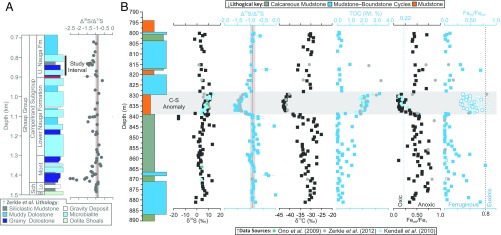
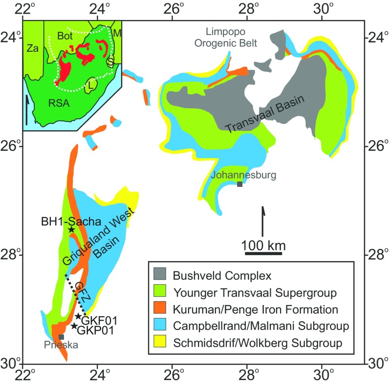
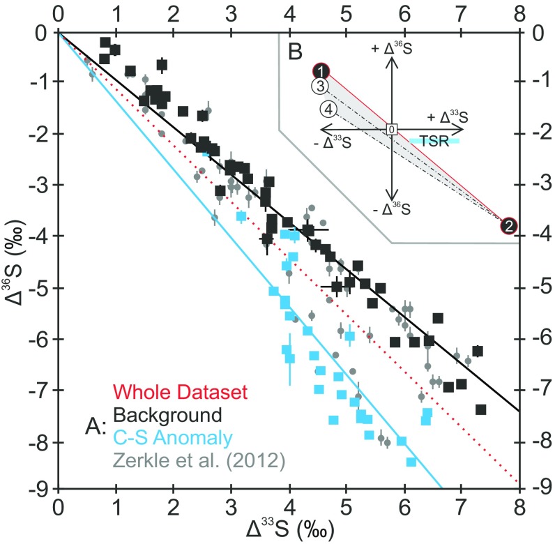
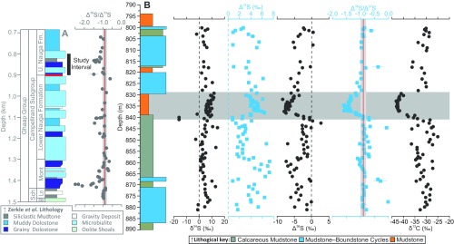
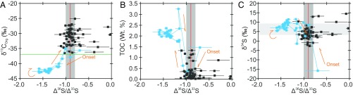
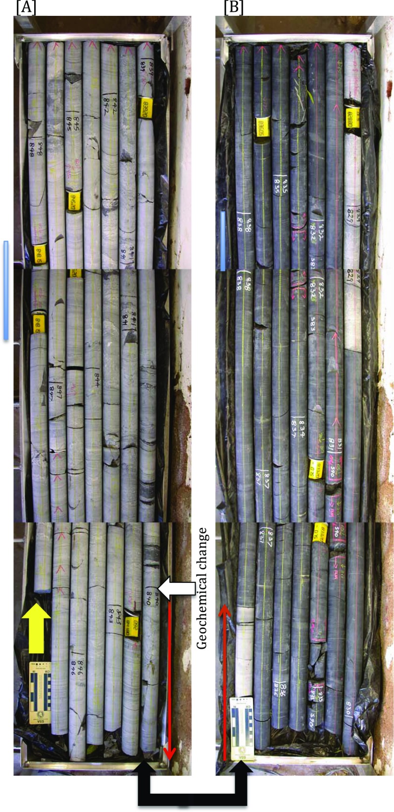
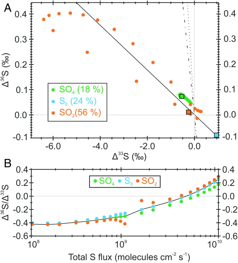
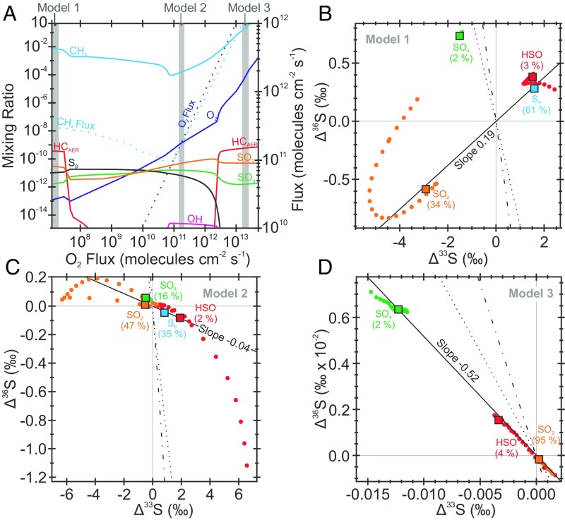
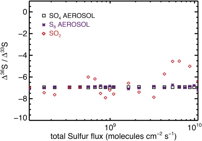
Emerging evidence suggests that atmospheric oxygen may have varied before rising irreversibly ∼2.4 billion years ago, during the Great Oxidation Event (GOE). Significantly, however, pre-GOE atmospheric aberrations toward more reducing conditions-featuring a methane-derived organic-haze-have recently been suggested, yet their occurrence, causes, and significance remain underexplored. To examine the role of haze formation in Earth's history, we targeted an episode of inferred haze development. Our redox-controlled (Fe-speciation) carbon- and sulfur-isotope record reveals sustained systematic stratigraphic covariance, precluding nonatmospheric explanations. Photochemical models corroborate this inference, showing Δ³⁶S/Δ³³S ratios are sensitive to the presence of haze. Exploiting existing age constraints, we estimate that organic haze developed rapidly, stabilizing within ∼0.3 ± 0.1 million years (Myr), and persisted for upward of ∼1.4 ± 0.4 Myr. Given these temporal constraints, and the elevated atmospheric CO₂ concentrations in the Archean, the sustained methane fluxes necessary for haze formation can only be reconciled with a biological source. Correlative δ¹³C_Org and total organic carbon measurements support the interpretation that atmospheric haze was a transient response of the biosphere to increased nutrient availability, with methane fluxes controlled by the relative availability of organic carbon and sulfate. Elevated atmospheric methane concentrations during haze episodes would have expedited planetary hydrogen loss, with a single episode of haze development providing up to 2.6-18 × 10¹⁸ moles of O₂ equivalents to the Earth system. Our findings suggest the Neoarchean likely represented a unique state of the Earth system where haze development played a pivotal role in planetary oxidation, hastening the contingent biological innovations that followed.

Keywords: Neoarchean; hydrogen loss; organic haze; planetary oxidation; sulfur mass-independent fractionation.

Fig. 1.

Preexisting lithological and geochemical data from core GKF01 (9) combined with new high-resolution geochemical data. (A) The published low-resolution GKF01 Δ³⁶S/Δ³³S record (9), the Neoarchean reference array (red line), and its ±0.1 uncertainty envelope (gray vertical band; ref. 8). (B) The new δ³⁴S, Δ³⁶S/Δ³³S, δ¹³C, TOC, and Fe-speciation (Fe_HR/Fe_T, Fe_Py/Fe_HR) data (squares) along with published data (filled circles; refs. , , and 24). The horizontal gray band signifies the C-S anomaly (discussed in the text). The vertical red line and gray envelope in the Δ³⁶S/Δ³³S plot represent the Neoarchean reference array and its associated uncertainty (± 0.1; ref. 8). Vertical lines in the Fe-speciation plots distinguish oxic from anoxic (Fe_HR/Fe_T ≥ 0.38) and ferruginous from definitively euxinic (Fe_Py/Fe_HR > 0.7) water column conditions. The open symbols in the Fe_HR/Fe_Py plot have Fe_HR/Fe_T <0.22, signifying oxic sedimentation (9, 15, 67). Assimilating these observations, sedimentation during the examined interval was likely dynamic, with a generally ferruginous background state (Fe_HR/Fe_T >0.38; Fe_Py/Fe_HR <0.7), becoming oxygenated during the C-S anomaly (Fe_HR/Fe_T <0.22; ref. 15). The definition of Fe_HR, Fe_Py, and Fe_T are given as a footnote to the text in Constraining the Timing and Drivers of Atmospheric Haze Formation, whereas the derivation of the diagnostic Fe-speciation threshold values are given in Methodology, Sedimentary Fe Speciation. Analytical uncertainties (1 SD, 1σ) are typically encompassed within each individual data point with the exception of a few Δ³⁶S/Δ³³S ratios whose uncertainty was computed from larger of the internal or external 1σ uncertainties associated with the raw Δ³³S and Δ³⁶S data (9). The large-scale lithological log (A) follows that presented in Zerkle et al. (9), whereas the new data (B) are plotted against the detailed sedimentary logs, which along with core photos are available online (general.uj.ac.za/agouron/index.aspx).

Fig. S1.

Geological map of the Transvaal Supergroup preserved on the Kaapvaal Craton with a geographical insert, modified from refs. and . The position of cores where Δ³⁶S/Δ³³S–δ¹³C covariation has been previously reported (core GKF01, ref. ; core BH1-Sacha, ref. 8) is indicated by labeled stars. Additionally the extra Agouron core (GKP01) that we discuss below in terms of chronological constraints is also given. The shallow-water Ghaap plateau facies are separated from their deep-water equivalents by the fault at Griquatown (GFZ; refs. and 53), hence the different stratigraphic nomenclature between Zerkle et al. (9) and Izon et al. (8).

Fig. 2.

Quadruple S-isotope data from core GKF01 (A) with a schematic mixing scenario (B). Δ³⁶S vs. Δ³³S trends for the new data (black and blue) superimposed on previously published data (gray circles; ref. 9). Regressions are given through the whole dataset (red) as well as through the C-S anomaly (blue) and background (black). Uncertainties are plotted conservatively, using the larger of the internal or external uncertainty (1σ), and are consistently smaller than a single data point. The insert (B) schematically illustrates the range of Δ³³S and Δ³⁶S values that can be expressed in pyrite (shaded gray area) formed via mixing of sulfide derived from MSR (open circles 3–4) with atmospherically derived S-MIF carried by sulfate (filled circle 1) and elemental sulfur (filled circle 2). The horizontal blue bar illustrates the Δ³⁶S-Δ³³S systematics of TSR derived sulfide. Note, biological activity has the potential to exert greater influence on Δ³⁶S/Δ³³S when pyrite carries a negative Δ³³S (i.e., derived from sulfate) rather than a positive Δ³³S (29) as observed in the C-S anomaly (Fig. 1). Additionally, mixing with TSR-derived sulfide moves the Δ³⁶S/Δ³³S to less negative values.

Fig. S2.

A depicts the stratigraphic distribution of the preexisting data (9) and B illustrates the new S- and C-isotope data (δ³⁴S, Δ³³S, Δ³⁶S, Δ³⁶S/Δ³³S, and δ¹³C_Org). The horizontal gray band illustrates the C-S anomaly, whereas the vertical red lines and their gray envelopes depict the Neoarchean reference array and its associated uncertainty (8). Analytical uncertainties are generally encompassed within individual datapoints, whereas uncertainty on the Δ³⁶S/Δ³³S ratio is computed from the larger of the internal or external uncertainties for Δ³⁶S and Δ³³S. Note the C-S anomaly predates the lithological change (see also Fig. S3).

Fig. 3.

Carbon isotope (δ¹³C) (A), TOC (B), and δ³⁴S (C) vs. Δ³⁶S/Δ³³S data from 800- to 900-m core depth in core GKF01. In each plot the data have been color-coded, differentiating the background (black) from the C-S anomaly (blue), with orange arrows illustrating its temporal evolution. Vertical red lines in each plot give the average Neoarchean Δ³⁶S/Δ³³S with a ±0.1 uncertainty envelope (vertical gray bar; ref. 8). The horizontal green line in A marks δ¹³C = −37‰, a threshold commonly used to identify methanotrophy (8, 9, 26). The horizontal gray bar in C represents the range of seawater δ³⁴S estimates derived from carbonate associated sulfate (55). Typically analytical uncertainty is encompassed within the data points, with the exception of a few Δ³⁶S/Δ³³S ratios as in Fig. 2.

Fig. S3.

Initial core photographs corresponding to the onset of the C-S anomaly. The cores become progressively younger up the page, as signaled by the bold yellow arrow and initial core markings. The older (deeper) core tray (A) is joined to the younger (shallower) tray B by the bold black arrows. The onset of the C-S anomaly (in both Δ³⁶S/Δ³³S and δ¹³C) is seen by 840-m core depth (annotated), whereas the change in lithology (from calcareous mudstone to mudstone) occurs at least 1 m up-core, in younger rocks. Thin red arrows highlight this nontrivial stratigraphic difference. Core photographs and detailed lithological logs of cores GKF01 and GKP01 are available via the Agouron-Griqualand Paleoproterozoic drilling project online database (general.uj.ac.za/agouron/index.aspx). These photos feature overlap (core markings and vertical blue boxes), and hence repetition of strata, to ensure the entire core was imaged.

Fig. 4.

Photochemical Δ³⁶S and Δ³³S predictions for the “standard atmosphere” (7) under normal conditions (A) and with differential sulfur loading (B). Under standard atmospheric conditions, in A sulfur leaves the model atmosphere unequally divided between three exit channels (SO₂, 56%; S₈, 24%; and SO₄, 18%). Values of Δ³⁶S/Δ³³S are displayed for the entire troposphere (filled circles), with the large squares showing the ground-level signal carried by a specific exit channel combining both wet and dry deposition. B recreates the experiment illustrated in figures 6 C and D in Claire et al. (7), where the total volcanic sulfur flux to the model atmosphere is varied over two orders of magnitude (10⁸–10¹⁰ molecules⁻² s⁻¹). The spatial distribution of atmospherically important species within the standard atmospheric framework is displayed in figure 2 of Claire et al. (7), where the following boundary conditions were adopted: volcanic sulfur flux of 3.85 × 10⁹ molecules⁻² s⁻¹ (∼1 Tmole y⁻¹) at an H₂S:SO₂ ratio of 1:10 and a volcanic H₂ flux of 1 × 10¹⁰ molecules⁻² s⁻¹ (∼3 Tmole y⁻¹). Fixed ground-level mixing ratios of 100 ppm and 10 ppb for CH₄ and O₂, respectively. Carbon dioxide concentrations were fixed at 1% at all heights, and N₂ provided a total atmospheric pressure of 1 bar. Full details of the model, validation, and its limitations are appended (Methodology, Photochemical Modeling).

Fig. 5.

Simulated Δ³⁶S/Δ³³S response to varying O₂ and CH₄ fluxes. (A) The three distinct atmospheric states (models 1–3, B–D) that were chosen to examine the effect of a hydrocarbon haze on atmospheric chemistry (numbered vertical gray bands in A). The first model simulates a thick hydrocarbon haze before the advent of oxygenic photosynthesis (B), whereas the second and third models represent haze-free (C) and hazy (D) states after the advent of oxygenic photosynthesis (7, 10). Under each atmospheric regime (B–D) the Δ³⁶S/Δ³³S carried by each atmospheric exit channel, at specific atmospheric height, is plotted as color-coded circles, whereas the atmospherically integrated signal (the ground-level value) of each vector is represented by a color-coded square. The relative importance of each exit channel is given in parentheses. In A the mixing ratios of atmospheric species are shown as solid lines (left axis), and fluxes are shown as dashed lines (right axis). In B–D the Archean reference array (Δ³⁶S/Δ³³S = −0.9; ref. 8), the steepened slope reflecting the C-S anomaly (Fig. 1) and the best fit to the simulated data are given by the dotted, dot-dashed, and solid lines, respectively. Full details of the model, validation, and its limitations are given in Methodology, Photochemical Modeling. Zero Δ³⁶S and Δ³³S data are given as gray lines to illustrate the change in scale between B–D.

Fig. S4.

Model validation of the updated photochemical model presented herein. Here, multiple simulations have been run with variable atmospheric sulfur loading, with only mass-dependent fractionation factors included. Integrated over the whole atmospheric reaction pathway, the average Δ³⁶S/Δ³³S carried by sulfur (SO₄) aerosols, octasulfur (S₈) aerosols, and sulfur dioxide (SO₂) are given by black squares, purple crosses, and red diamonds, respectively.

References

1. Farquhar J, Bao H, Thiemens M. Atmospheric influence of Earth’s earliest sulfur cycle. Science. 2000;289(5480):756–759. - PubMed
1. Farquhar J, Savarino J, Airieau S, Thiemens MH. Observation of wavelength-sensitive mass-independent sulfur isotope effects during SO2 photolysis: Implications for the early atmosphere. J Geophys Res Planets. 2001;106(E12):32829–32839.
1. Pavlov AA, Kasting JF. Mass-independent fractionation of sulfur isotopes in Archean sediments: Strong evidence for an anoxic Archean atmosphere. Astrobiology. 2002;2(1):27–41. - PubMed
1. Holland HD. The oxygenation of the atmosphere and oceans. Philos Trans R Soc Lond B Biol Sci. 2006;361(1470):903–915. - PMC - PubMed
1. Bekker A, et al. Dating the rise of atmospheric oxygen. Nature. 2004;427(6970):117–120. - PubMed
Publication types