Historical changes of the Mediterranean Sea ecosystem: modelling the role and impact of primary productivity and fisheries changes over time

Abstract

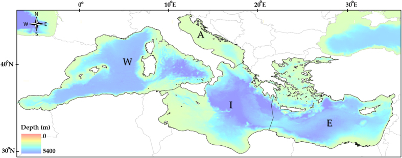
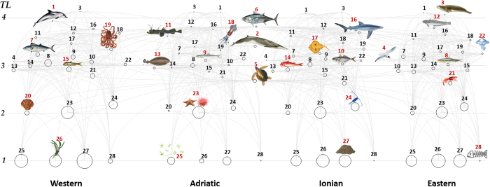
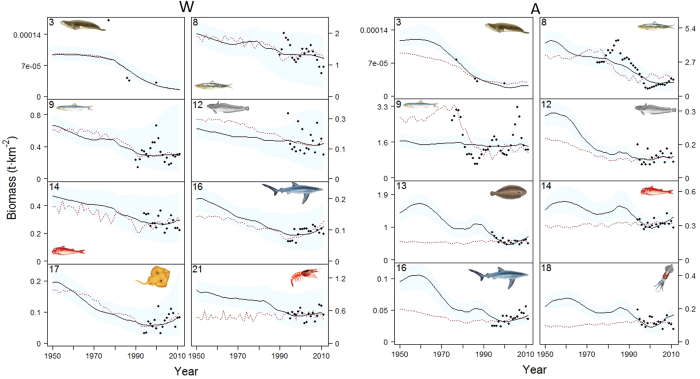
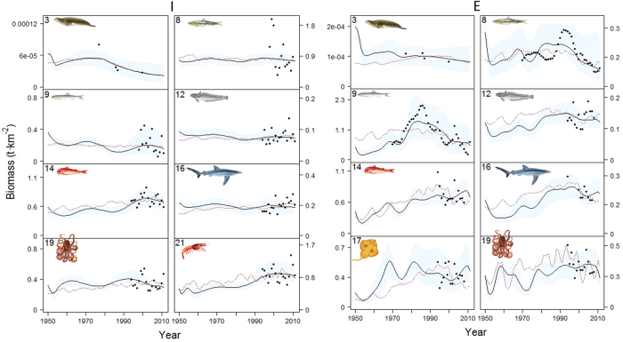
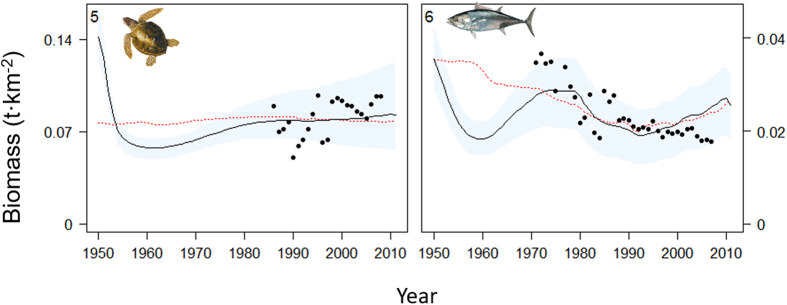
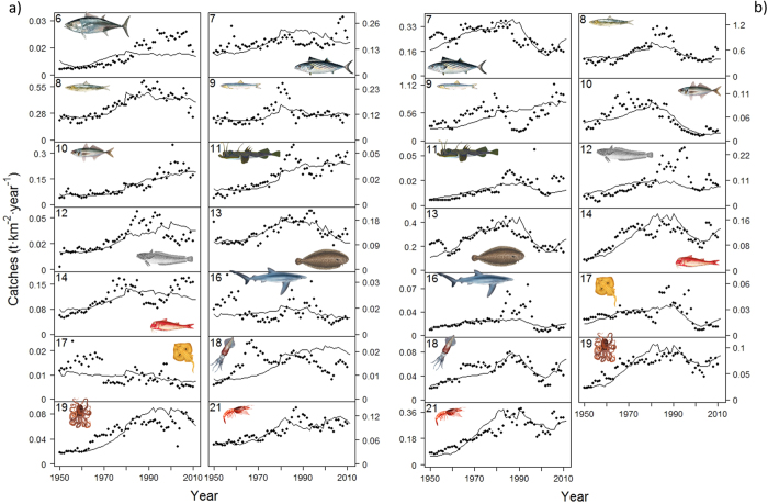
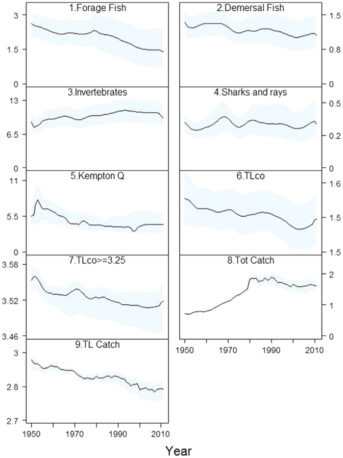
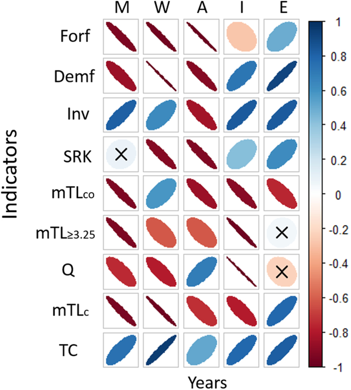
The Mediterranean Sea has been defined "under siege" because of intense pressures from multiple human activities; yet there is still insufficient information on the cumulative impact of these stressors on the ecosystem and its resources. We evaluate how the historical (1950-2011) trends of various ecosystems groups/species have been impacted by changes in primary productivity (PP) combined with fishing pressure. We investigate the whole Mediterranean Sea using a food web modelling approach. Results indicate that both changes in PP and fishing pressure played an important role in driving species dynamics. Yet, PP was the strongest driver upon the Mediterranean Sea ecosystem. This highlights the importance of bottom-up processes in controlling the biological characteristics of the region. We observe a reduction in abundance of important fish species (~34%, including commercial and non-commercial) and top predators (~41%), and increases of the organisms at the bottom of the food web (~23%). Ecological indicators, such as community biomass, trophic levels, catch and diversity indicators, reflect such changes and show overall ecosystem degradation over time. Since climate change and fishing pressure are expected to intensify in the Mediterranean Sea, this study constitutes a baseline reference for stepping forward in assessing the future management of the basin.

Figure 1. A representation of the Mediterranean Sea with the bathymetry and the four MSFD areas: Western Mediterranean Sea (W); Adriatic Sea (A); Ionian and Central Mediterranean Sea (I); Aegean and Levantine Sea (E).

Map was originated using the GIS (Geographical Information System; ArcMap version 10.3; www.esri.com) software.

Figure 2. Flow diagram of the Mediterranean Sea ecosystem (year 1950 s) with the Western part being at the far left followed by the Adriatic, the Ionian and the Eastern.

Each functional group is shown as a circle and its size is proportional to the log of its biomass. The functional groups are represented by their trophic levels (y-axis) and linked by predator-prey relationships showed as light grey lines. Numbers refer to functional group codes, which are reported in the legend, while those in red are graphically represented with a drawing. Numbers in the figure: 1. Piscivorous cetaceans; 2. Other cetaceans; 3. Pinnipeds; 4. Seabirds; 5. Sea turtles; 6. Large pelagics; 7. Medium pelagics; 8. European pilchard; 9. European anchovy; 10. Other small pelagics; 11. Large demersals; 12. European hake; 13. Medium demersals; 14. Small demersals; 15. Deep sea fish; 16. Sharks; 17. Rays and skates; 18. Benthopelagic cephalopods; 19. Benthic cephalopods; 20. Bivalves and gastropods; 21. Crustaceans; 22. Jellyfish; 23. Benthos; 24. Zooplankton; 25. Phytoplankton; 26. Seagrass; 27. Detritus; 28. Discards. Drawings for species/functional groups 1–3, 5–6 and 8 are by Massimo Demma - http://www.massimodemma.it/-.

Figure 3. Representation of modelling fitting results for some functional groups occurring in the Western and Adriatic Seas for the period 1950–2011 (results for the rest of the groups are shown in Figure S8)

Predicted biomass (t·km⁻²) is shown as solid black lines, while observed data is represented as black dots. Functional groups codes correspond to those given in Fig. 2. The predicted model (dashed red line) using modelled biogeochemical PP is also shown. Blue shadow represents the 95% percentile and 5% percentile obtained through the Monte Carlo routine. Drawings for species/functional groups 1–3, 5–6 and 8 are by Massimo Demma - http://www.massimodemma.it/-.

Figure 4. Representation of modelling fitting results for some functional groups occurring in the Ionian and Eastern Seas for the period 1950–2011 (results for the rest of the groups are shown in Figure S8).

Predicted biomass (t·km⁻²) is shown as solid black lines, while observed data is represented as black dots. Functional groups codes correspond to those given in Fig. 2. The predicted model (dashed red line) using modelled biogeochemical PP is also shown. Blue shadow represents the 95% percentile and 5% percentile obtained through the Monte Carlo routine. Drawings for species/functional groups 1–3, 5–6 and 8 are by Massimo Demma - http://www.massimodemma.it/-.

Figure 5. Representation of modelling fitting results for large pelagics and sea turtles in the Mediterranean Sea as whole for the period 1950–2011.

Predicted biomass (t·km⁻²) is shown as solid black lines, while observed data is represented as black dots. Functional groups codes correspond to those given in Fig. 2. The predicted model (dashed red line) using modelled biogeochemical PP is also shown. Blue shadow represents the 95% percentile and 5% percentile obtained through the Monte Carlo routine. Drawings for species/functional groups 1–3, 5–6 and 8 are by Massimo Demma - http://www.massimodemma.it/-.

Figure 6

Predicted (solid lines) versus observed (dots) catches (t·km⁻²·year⁻¹) for main commercially important functional groups of the Western Mediterranean (a) and Adriatic (b) ecosystems (1950–2011). Predictions obtained with the Mediterranean Sea model as whole for large pelagic catches are included in the Western Mediterranean plot (a. #6). Results for the Ionian and Aegean catches are shown in Figure S9. Drawings for species/functional groups 1–3, 5–6 and 8 are by Massimo Demma - http://www.massimodemma.it/-.

Figure 7. Ecological indicators 1.

Forage fish biomass (t·km⁻²); 2. Demersal fish biomass (t·km⁻²); 3. Invertebrates biomass (t·km⁻²); 4. Sharks/rays and skate biomass (t·km⁻²); 5. Kempton Q: Kempton’s index of biodiversity; 6. TLco: Mean trophic level of the community; 7. TLco ≥ 3.25: Mean trophic levels of groups having trophic level ≥ 3.25 (excluding marine mammals, sea turtles and seabirds); 8. Tot Catch: Total catch (t· km⁻² ·year-1); 9 TL Catch: Mean trophic level of the catches) estimated from the Ecosim results for the period 1950–2011 for the Catch Mediterranean Sea. Blue shadow represents the 95% percentile and 5% percentile obtained through the Monte Carlo routine.

Figure 8. Spearman’s rank-order correlations representation between the suite of ecological indicators (Forf: Forage fish biomass (t·km⁻²); Demf: Demersal fish biomass (t·km⁻²); Inv: Invertebrates biomass (t·km⁻²); SRK: Sharks/rays and skate biomass (t·km⁻²); mTLco: Mean trophic level of the community; mTL ≥ 3.25: Mean trophic levels of groups having trophic level >3.25 (excluding marine mammals, sea turtles and seabirds); Q: Kempton’s index of biodiversity; mTLc: Mean trophic level of the catches; TC: Total catch (t· km⁻² ·year⁻¹) and time for the four sub-areas (Western: W; Adriatic: A; Ionian: I; Eastern and Levantine: E) and for the additional Mediterranean Sea as whole (Mediterranean: M).

Positive correlations are displayed in blue and negative correlations in red color. Color intensity and the size of the eclipses are proportional to the correlation coefficients. At the right side of the graph, the legend color shows the correlation coefficients and the corresponding colors. The color follows a gradient according to the strength of the correlation. The width of the ellipses is related to correlation strengths with more diffused ellipses representing lower correlation strengths. When the indicators are non-significant (>0.05) are represented with an X symbol.

References

1. Halpern B. S. et al. A global map of human impact on marine ecosystems. Science 319, 948–952 (2008). - PubMed
1. Côté I. M., Darling E. S. & Brown C. J. Interactions among ecosystem stressors and their importance in conservation Proc. R. Soc. B. 20152592 (2016). - PMC - PubMed
1. Mora C. et al. Biotic and human vulnerability to projected changes in ocean biogeochemistry over the 21st century. PLoS Biol 11, e1001682 (2013). - PMC - PubMed
1. Halpern B. S. et al. Spatial and temporal changes in cumulative human impacts on the world’s ocean. Nature communications 6 (2015). - PMC - PubMed
1. Travers M. et al. Two-way coupling versus one-way forcing of plankton and fish models to predict ecosystem changes in the Benguela. Ecological modelling 220, 3089–3099 (2009).
Publication types