Review of interferometric spectroscopy of scattered light for the quantification of subdiffractional structure of biomaterials

Abstract

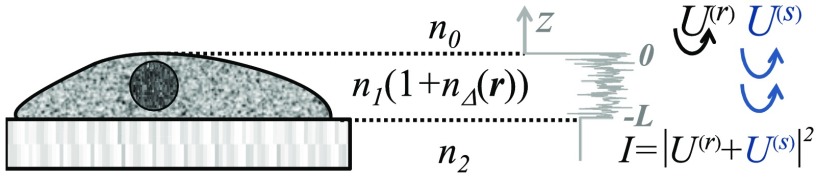
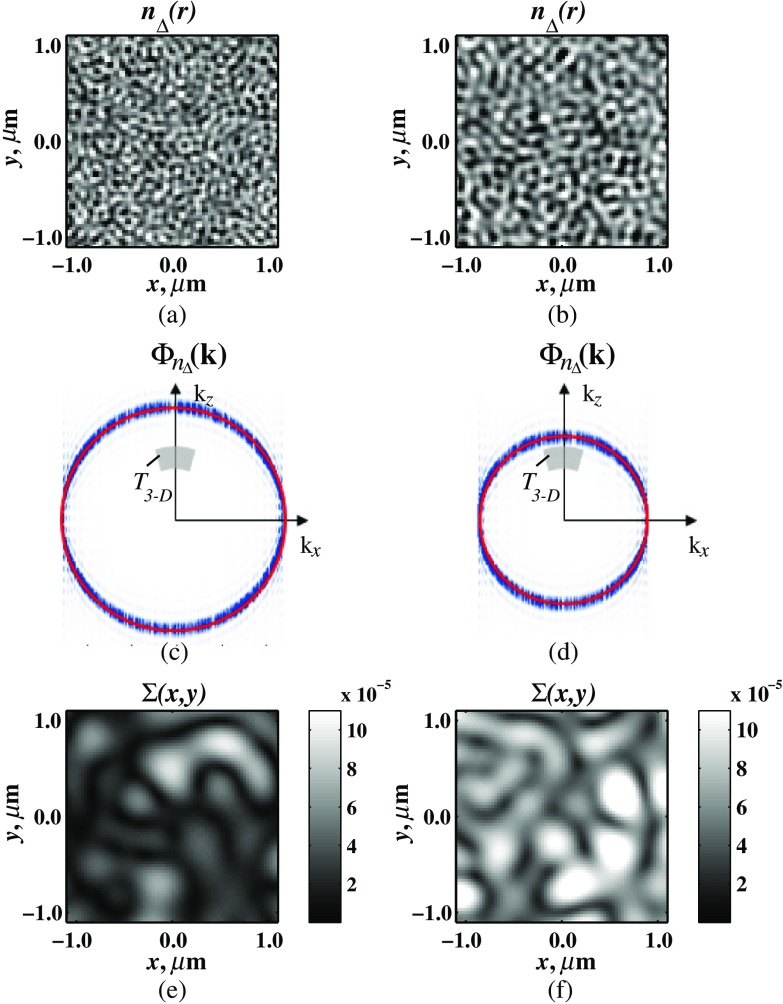
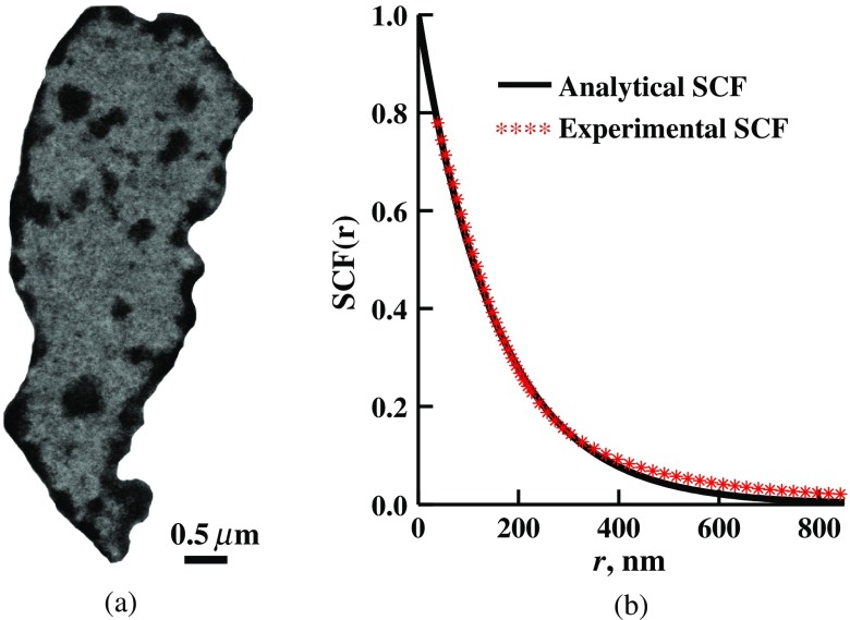
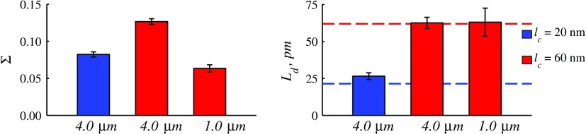
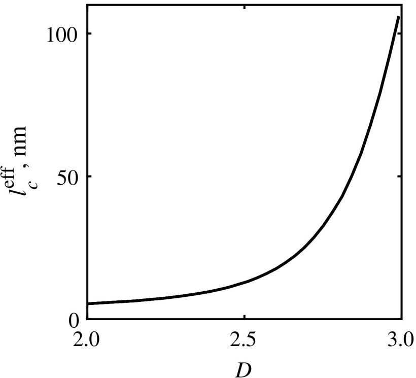
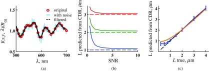
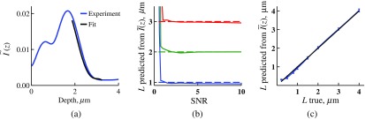
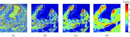
Optical microscopy is the staple technique in the examination of microscale material structure in basic science and applied research. Of particular importance to biology and medical research is the visualization and analysis of the weakly scattering biological cells and tissues. However, the resolution of optical microscopy is limited to ? 200 ?? nm due to the fundamental diffraction limit of light. We review one distinct form of the spectroscopic microscopy (SM) method, which is founded in the analysis of the second-order spectral statistic of a wavelength-dependent bright-field far-zone reflected-light microscope image. This technique offers clear advantages for biomedical research by alleviating two notorious challenges of the optical evaluation of biomaterials: the diffraction limit of light and the lack of sensitivity to biological, optically transparent structures. Addressing the first issue, it has been shown that the spectroscopic content of a bright-field microscope image quantifies structural composition of samples at arbitrarily small length scales, limited by the signal-to-noise ratio of the detector, without necessarily resolving them. Addressing the second issue, SM utilizes a reference arm, sample arm interference scheme, which allows us to elevate the weak scattering signal from biomaterials above the instrument noise floor.

Fig. 1

Sample: RI of the middle layer is random, RIs of the top and bottom layers are constant; RI as a function of depth is shown in gray. Coherent sum of $U^{(r)}$ and $U^{(s)}$ is detected. Reflection from the substrate (glass slide) is negligible as its thickness (1 mm) is much larger than the microscope’s depth of field. Reproduced with permission from Ref. , courtesy of J. Biomed. Opt.

Fig. 2

$B_{n_{\mathrm{\Delta }}}/{\sigma }_{n_{\mathrm{\Delta }}}^2$ versus $D$ for $L_n=0.5\mu \mathrm{m}$ (dashed lines) and $L_n=1.5\mu \mathrm{m}$ (solid lines). Horizontal black line indicates the level at which correlation decays by a factor of $e$.

Fig. 3

Spatial-frequency space with $k_z$-axis antiparallel to ${\mathbf{k}}_i$. (a) Cross section of $T_{\mathrm{\Delta }{\mathbf{k}}_{\mathbf{s}}}$, $T_{k\mathrm{NA}}$, and their interception, $T_{3\text{-}\mathrm{D}}$; (b) PSD of the RI fluctuation (blue) and $T_{3\text{-}\mathrm{D}}$ (gray) when the sample can be considered infinite (i.e., the LSs of internal organization are much smaller than sample thickness $L$); and (c) when the sample is finite. Reproduced with permission from Ref. , courtesy of Phys. Rev. Lett.

Fig. 4

$\tilde{\mathrm{\Sigma }}$ for $D\in (\mathrm{2,4})$ for samples with (a) $L=0.5\mu \mathrm{m}$ and (b) $L=2\mu \mathrm{m}$ shows a monotonic increase with $D$ and a negligible dependence on the correlation outer scale $L_n$. The dependence on $D$ for $L_n\in (0.5,1.5)\mu \mathrm{m}$ explained in terms of the effective correlation length $l_c^{\mathrm{eff}}$ in case of (c) $L=0.5\mu \mathrm{m}$ and (d) $L=2\mu \mathrm{m}$.

Fig. 5

Cross section of single spatial-frequency medium with $1/k_{\mathrm{LS}}$ of (a) 15 and (b) 20 nm ($k_{\mathrm{LS}}$ evaluated in vacuum). Cross section of PSD of an infinite (red) and thin ($L=0.5\mu \mathrm{m}$) media with $1/k_{\mathrm{LS}}$ of (c) 15 and (d) 20 nm. The sensitivity of $\tilde{\mathrm{\Sigma }}$ to periodic structures with subdiffractional frequencies illustrated in the clear difference in the value of $\mathrm{\Sigma }(x,y)$ corresponding to the media with $1/k_{\mathrm{LS}}$ of (e) 15 and (f) 20 nm. Note that the subdiffractional structures are not resolved in the diffraction-limited $\mathrm{\Sigma }(x,y)$ image.

Fig. 6

$\tilde{\mathrm{\Sigma }}/{\sigma }_{n_{\mathrm{\Delta }}}{R}_{01}^2$ as a function of the spatial frequency of RI fluctuations for samples with different thicknesses (all wavenumbers evaluated in vacuum). Reproduced with permission from Ref. , courtesy of Opt. Lett.

Fig. 7

Dependence of $\tilde{\mathrm{\Sigma }}$ on changes in LS composition. Cross sections of a media with two LSs: (a) 20 and 200 nm (b) 40 and 200 nm (representing a twofold change in the smaller LS), and (c) 40 and 400 nm (representing a twofold change in the larger length scale). (d) $\tilde{\mathrm{\Sigma }}$ that would be measured from the corresponding samples with $L=3\mu \mathrm{m}$, bars are standard deviations between 10 samples per statistical condition.

Fig. 8

Dependence of (a) $r_{\min }$ and (b) $r_{\max }$ corresponding to the 5% threshold on $L$ and $l_c$. Black dashed lines indicate $r_{\min }=22\mathrm{nm}$ and $r_{\max }=171\mathrm{nm}$ corresponding to $L=\infty$. Reproduced with permission from Ref. , courtesy of Opt. Lett.

Fig. 9

(a) Example TEM image of a human colonic cell nucleus. (b) Experimental SCF obtained as average of SCFs measured from 36 nuclei (defined only at $r>39\mathrm{nm}$) and the analytical fit to it.

Fig. 10

Relative change in $\tilde{\mathrm{\Sigma }}$ when (a) lower (${\tilde{\mathrm{\Sigma }}}^l/\tilde{\mathrm{\Sigma }}$) and (b) higher (${\tilde{\mathrm{\Sigma }}}^h/\tilde{\mathrm{\Sigma }}$) LSs are perturbed. Calculation performed for samples with SCF that is experimentally measured from TEM images (blue markers for samples with thickness $1.5\mu \mathrm{m}$ and green for $6.0\mu \mathrm{m}$), and analytically defined as exponential (blue solid line for $L=1.5$ and green dashed for $L=6.0\mu \mathrm{m}$). Reproduced with permission from Ref. , courtesy of Opt. Lett.

Fig. 11

Schematic of an example SM instrument. White light is incident from a lamp using Kohler illumination microscope light path (KI Optics) through the objective (OBJ) onto the sample. Spectrally resolved microscope image is registered on a charge coupled device camera using a spectral filter (SF, either a slit spectrometer or a liquid-crystal tunable filter). TL denotes a tube lens, and BS denotes a beam splitter. Spectrally resolved image acquisition can be obtained by placing a tunable SF (a) either in front of the light source and scanning the wavelength of the illumination light or (b) in front of the camera and scanning the wavelength of the microscope image. For option (b), one also uses a slit spectrometer and scan the sample plane to form a wavelength-resolved image.

Fig. 12

$\tilde{\mathrm{\Sigma }}(l_c)$ for various values of ${\mathrm{NA}}_i$ between 0 and 0.6 for SM images synthesized by FDTD from samples with $L=500\mathrm{nm}$. No significant dependence on ${\mathrm{NA}}_i$ of $\tilde{\mathrm{\Sigma }}(l_c)$ is observed for ${\mathrm{NA}}_i<0.4$.

Fig. 13

(a) ${\tilde{\mathrm{\Sigma }}}_R(l_c)$, (b) ${\tilde{\mathrm{\Sigma }}}_L(l_c)$, and (c) $\tilde{\mathrm{\Sigma }}(l_c)$ as a function of the NA of light collection for a sample with $L=2\mu \mathrm{m}$.

Fig. 14

Reference-arm reflectance, calculated as the average spectrum across image pixels $(x,y)$ for various standard deviations of height within a diffraction-limited area ${\sigma }_h$ between 10 and 50 nm. Reproduced with permission from Ref. , courtesy of Opt. Lett.

Fig. 15

Bright-field epi-illumination microscope images of inhomogeneous samples with $L=2\mu \mathrm{m}$ (a) $l_c=20\mathrm{nm}$ and a smooth surface, (b) $l_c=100\mathrm{nm}$ and a smooth surface, (c) $l_c=100\mathrm{nm}$ and a rough surface with standard deviation of height variations ${\sigma }_h=36\mathrm{nm}$. Corresponding $\mathrm{\Sigma }(x^{\prime },y^{\prime })$ images, (d) $l_c=20\mathrm{nm}$ and a smooth surface, (e) $l_c=100\mathrm{nm}$ and a smooth surface, (f) $l_c=100\mathrm{nm}$ and a rough top surface. ${\mathrm{\Sigma }}^{\prime }(x^{\prime },y^{\prime })$ images, obtained after a second-order polynomial subtraction from detected spectra, are shown in panels (g)–(i) correspondingly. (j) Example spectra for $l_c=20\mathrm{nm}$ smooth (black), $l_c=100\mathrm{nm}$ smooth (red), and $l_c=100\mathrm{nm}$ rough (blue). (k) Average $\tilde{\mathrm{\Sigma }}$ and for the above samples, 10 samples per statistical condition. (l) Average ${\tilde{\mathrm{\Sigma }}}^{\prime }$ and for the above samples, 10 samples per statistical condition eighth error bars corresponding to standard deviations. Scale bar 300 nm on all panels.

Fig. 16

(a) Comparison between true $L_d$ and that predicted from an SM measurement $\tilde{\mathrm{\Sigma }}$ for samples with various thickness values ranging from 0.5 to $4\mu \mathrm{m}$. (b) Comparison between true $D$ and that predicted from an SM measurement $\tilde{\mathrm{\Sigma }}$ for samples with $L$ from 0.5 to $4\mu \mathrm{m}$, $L_n=1\mu \mathrm{m}$ (solid lines), and $L_n=2\mu \mathrm{m}$ (dashed lines).

Fig. 17

Finding $L_d=l_c{\sigma }_{n_{\mathrm{\Delta }}}^2$ from $\tilde{\mathrm{\Sigma }}$ for samples with nanoscale $l_c$ of 20 and 60 nm and very different thicknesses.

Fig. 18

Increase in the effective correlation length $l_c^{\mathrm{eff}}$ with the fractal dimension $D$. Here, $L_n=1\mu \mathrm{m}$.

Fig. 19

(a) Example spectrum for $L=3\mu \mathrm{m}$, $l_c=34\mathrm{nm}$ originally simulated by FDTD (red), with added noise to imitate experimental conditions in the case of poor $\mathrm{SNR}=2$ (cyan), and after applying low-pass frequency filter to remove noise (black dashed). The filtered signal approximates the original with 2% accuracy and is used for further CDR calculations. (b) Thickness predicted from CDR for various SNR (solid lines in red for $L=3\mu \mathrm{m}$, green for $L=2\mu \mathrm{m}$, blue for $L=1\mu \mathrm{m}$). True sample thickness is indicated by dashed lines of the corresponding color. (c) Thickness predicted from CDR at $\mathrm{SNR}=10$ measured from FDTD-simulated spectra (blue) as well as predicted theoretically (orange) for a wide range of true sample thicknesses.

Fig. 20

(a) Example Fourier transform of spectrum for $L=2\mu \mathrm{m}$, generated by FDTD (blue) and the decay fit (black). (b) Thickness predicted from decay tail for various SNR (solid lines in red for $L=3\mu \mathrm{m}$, green for $L=2\mu \mathrm{m}$, blue for $L=1\mu \mathrm{m}$). True sample thickness is indicated by dashed lines of the corresponding color. (c) Thickness predicted from decay tail measured from FDTD-simulated spectra for a wide range of true sample thicknesses.

Fig. 21

$L(x,y)$ of a fixed prostate tissue section ($\mu \mathrm{m}$) calculated using: (a) thickness reconstruction from CDR considering every pixel independently, and (b) applying a median filter with a window size of a diffraction-limited spot, pixels with SNR $<1$ excluded, (c) thickness reconstruction using frequency-spectral decay, and (d) atomic force microscopy measurements. Panels c-d reproduced with permission from Ref. , courtesy of J. Biomed. Opt.

Fig. 22

(a) ${\tilde{\mathrm{\Sigma }}}_R/\sqrt{k_{c}L}$ and ${\tilde{\mathrm{\Sigma }}}_L$ as a function of the correlation length $l_c$ obtained for a sample with thickness $L=2\mu \mathrm{m}$ according to analytical equations (solid lines) and calculated from FDTD simulation (circles with error bars corresponding to the standard deviation between nine ensembles per statistical condition). (b) Corresponding true ${\sigma }_{n_{\mathrm{\Delta }}}$ and $l_c$ (solid lines) and reconstructed from FDTD-synthesized SM signal (circles with error bars corresponding to the standard deviation between nine ensembles per statistical condition). Reproduced with permission from Ref. , courtesy of J. Biomed. Opt.

References

1. Itzkan I., et al. , “Confocal light absorption and scattering spectroscopic microscopy monitors organelles in live cells with no exogenous labels,” Proc. Natl. Acad. Sci. U. S. A. 104(44), 17255–17260 (2007).10.1073/pnas.0708669104 - DOI - PMC - PubMed
1. Alexandrov S. A., et al. , “Spectral encoding of spatial frequency approach for characterization of nanoscale structures,” Appl. Phys. Lett. 101(3), 033702 (2012).APPLAB10.1063/1.4737209 - DOI - PMC - PubMed
1. Alexandrov S., Sampson D., “Spatial information transmission beyond a system’s diffraction limit using optical spectral encoding of the spatial frequency,” J. Opt. A: Pure Appl. Opt. 10(2), 025304 (2008).10.1088/1464-4258/10/2/025304 - DOI
1. Alexandrov S. A., et al. , “Novel approach for label free super-resolution imaging in far field,” Sci. Rep. 5, 13274 (2015).10.1038/srep13274 - DOI - PMC - PubMed
1. Joo C., et al. , “Spectral-domain optical coherence phase microscopy for quantitative phase-contrast imaging,” Opt. Lett. 30(16), 2131–2133 (2005).OPLEDP10.1364/OL.30.002131 - DOI - PubMed