The connective tissue phenotype of glaucomatous cupping in the monkey eye - Clinical and research implications

Abstract

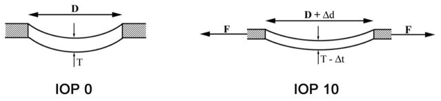
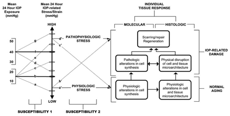
In a series of previous publications we have proposed a framework for conceptualizing the optic nerve head (ONH) as a biomechanical structure. That framework proposes important roles for intraocular pressure (IOP), IOP-related stress and strain, cerebrospinal fluid pressure (CSFp), systemic and ocular determinants of blood flow, inflammation, auto-immunity, genetics, and other non-IOP related risk factors in the physiology of ONH aging and the pathophysiology of glaucomatous damage to the ONH. The present report summarizes 20 years of technique development and study results pertinent to the characterization of ONH connective tissue deformation and remodeling in the unilateral monkey experimental glaucoma (EG) model. In it we propose that the defining pathophysiology of a glaucomatous optic neuropathy involves deformation, remodeling, and mechanical failure of the ONH connective tissues. We view this as an active process, driven by astrocyte, microglial, fibroblast and oligodendrocyte mechanobiology. These cells, and the connective tissue phenomena they propagate, have primary and secondary effects on retinal ganglion cell (RGC) axon, laminar beam and retrolaminar capillary homeostasis that may initially be "protective" but eventually lead to RGC axonal injury, repair and/or cell death. The primary goal of this report is to summarize our 3D histomorphometric and optical coherence tomography (OCT)-based evidence for the early onset and progression of ONH connective tissue deformation and remodeling in monkey EG. A second goal is to explain the importance of including ONH connective tissue processes in characterizing the phenotype of a glaucomatous optic neuropathy in all species. A third goal is to summarize our current efforts to move from ONH morphology to the cell biology of connective tissue remodeling and axonal insult early in the disease. A final goal is to facilitate the translation of our findings and ideas into neuroprotective interventions that target these ONH phenomena for therapeutic effect.

Keywords: Astrocyte; Glaucoma; Lamina cribrosa; Monkey; Optic nerve head.

Figure 1. Optic Nerve Head (ONH) Homeostasis is Influenced by Intraocular Pressure (IOP)-related Stress and Strain at all levels of IOP

See Section 2.2 for details. (A) Prelaminar, laminar and retrolaminar ONH regions. (B) The clinically visible surface of the normal ONH (referred to as the optic disc). Central retinal vessels enter the eye and RGC axons appear pink due to their capillaries. (C) The posterior ciliary arteries (PCA) are the principal blood supply to the ONH (see Figures 4 and 5). (D) The lamina cribrosa (LC) is (schematically depicted with axon bundles in (D), isolated by trypsin digest in a scanning electron micrograph in (E) and drawn with stippled extracellular matrix (ECM), central capillary (red) and surrounding astrocytes (yellow with basement membranes in black) (F). The clinical manifestation of IOP-induced damage to the ONH is most commonly “deep cupping” (G) but in some eyes cupping can be shallower accompanied by pallor (H). Z-H = circle of Zinn-Haller; PCA= posterior ciliary arteries; NFL = nerve fiber layer; PLC = prelaminar region; LC = lamina cribrosa; RLC = retrolaminar region; ON = optic nerve; CRA = central retinal artery. A - Reproduced with permission from Arch Ophthalmol.1969;82:800–814. Copyright © (1969) American Medical Association. All rights reserved (Anderson and Hoyt, 1969). B, G, H – Reprinted from J Glaucoma. 2008;17(4):318–28, with permission from Wolters Kluwer Health, Inc. (Burgoyne and Downs, 2008). C - Reprinted courtesy of J. Cioffi and M. Van Buskirk, from The Glaucomas. St. Louis, Mosby: Basic Sciences; 1996:177–197 (Cioffi and Van Buskirk, 1996). D –Reprinted courtesy of Harry Quigley, from Optic Nerve in Glaucoma. Amsterdam: Kugler Publications; 1995:15–36(Quigley, 1995b). E - Reproduced with permission from Arch Ophthalmol. 1990;108:51–57. Copyright © (1990) American Medical Association. All rights reserved (Morrison et al., 1989). F - Reproduced with permission from Arch Ophthalmol. 1989;107:123–129. Copyright © (1989) American Medical Association. All rights reserved (Quigley et al., 1990).

Figure 2. Principle distribution of forces, pressures and the translaminar pressure gradient within the optic nerve head (ONH)

See section 2.3 for details. (A) Cut-away diagram of intraocular pressure (IOP)-induced mechanical stress in an idealized spherical scleral shell. Red arrows: IOP/orbital pressure difference; Green arrows: peripapillary scleral hoop stress generated by IOP; Blue arrows: peripapillary tensile stress that is generated by the lamina and delivered to the laminar beams. (B) Pink arrows: retrolaminar tissue pressure (RLTP) which is higher than cerebrospinal fluid pressure (Yellow arrows). C. The difference between IOP and the retrolaminar tissue pressure is the translaminar pressure difference which generates both a net posterior (outward) force on the surface of the lamina (the red arrows over the lamina) and a hydrostatic pressure gradient (the translaminar pressure gradient - schematically shown in green) within the neural and connective tissues of the pre-laminar and laminar regions. Panel A - Adapted from Downs JC, Roberts MD, Burgoyne CF. Mechanical Strain and Restructuring of the Optic Nerve Head. In: Shaarawy T, Sherwood MB, Hitchings RA, Crowston JG, editors. Glaucoma. 1 ed. London: Saunders, Copyright 2009, with permission from Elsevier (Downs et al., 2009). Panels B & C - Reprinted from Exp Eye Res, 93(2), Burgoyne CF, A biomechanical paradigm for axonal insult within the optic nerve head in aging and glaucoma, 120–32, Copyright 2011, with permission from Elsevier (Burgoyne, 2011).

Figure 3. Schematic Representation of the Laminar/Scleral Dynamic as Experimentally Observed in Non-pressurized (Intraocular Pressure (IOP) 0, left) and pressurized (IOP 10, right) Monkey Control Eyes (Bellezza et al., 2003a)

See Section 2.4 for details. (Left): Thickness (T) of the lamina cribrosa and diameter (D) of the scleral canal opening in an unpressurized (IOP 0) eye. (Right): Pressure within the globe generates an expansion of the scleral shell which, in turn, generates (and is resisted by) tensile forces within the sclera. These forces (F) act on the scleral canal wall, causing the scleral canal opening to expand (Δd), which in turn stretches the lamina within the canal. Thus, the lamina is taut (more anteriorly positioned) and thinned (Δt) in the IOP 10 eye, compared with the IOP 0 eye. Reproduced from Br J Ophthalmol, Bellezza AJ, Rintalan CJ, Thompson HW, Downs JC, Hart RT, Burgoyne CF. Anterior scleral canal geometry in pressurised (IOP 10) and non-pressurised (IOP 0) normal monkey eyes, 87(10):1284–90, copyright 2003 with permission from BMJ Publishing Group Ltd (Bellezza et al., 2003a).

Figure 4. The Volume Flow of Blood within the Posterior Ciliary Arteries should be affected by Intraocular Pressure (IOP)-related Stress and Strain within the Peripapillary Sclera (pp-sclera) and Scleral Flange

See Section 2.5 for details. The posterior ciliary arteries pass through the pp-sclera (yellow, left and center panel) immediately adjacent to the scleral portion of the neural canal. We refer to this portion of the sclera as the scleral flange (Yang et al., 2007b) (yellow arrows, middle figure). Each laminar beam contains a capillary (Panel F, Figure 1) which are here shown in a vascular casting of a monkey eye (Cioffi and Van Buskirk, 1996). Left and right panels reprinted courtesy of J. Cioffi and M. Van Buskirk, from The Glaucomas. St. Louis, Mosby: Basic Sciences; 1996:177–197 (Cioffi and Van Buskirk, 1996). Middle Panel reprinted from Exp Eye Res, 93(2), Burgoyne CF, A biomechanical paradigm for axonal insult within the optic nerve head in aging and glaucoma, 120–32, Copyright 2011, with permission from Elsevier (Burgoyne, 2011).

Figure 5. Hayreh (Hayreh et al., 1970) demonstrated Sensitivity of the Peripapillary Choroidal Circulation (green) to Acute Intraocular Pressure (IOP) elevation in the Monkey Optic Nerve Head (ONH)

See Section 2.5 for details. Fluorescence fundus angiogram of the right eye of a cynomologus monkey after experimental central retinal artery occlusion at normal (far left) and 70 mm Hg IOP (middle left and right). The non-perfused region of the peripapillary choroid is schematically highlighted in green (middle right). We and others have hypothesized that IOP-related stress and strain within the scleral flange (Figure 4, above) may contribute to this phenomenon and that similar effects may occur within the laminar capillary beds (red) (middle and far right). The far right panel is reprinted courtesy of J. Cioffi and M. Van Buskirk, from The Glaucomas. St. Louis, Mosby: Basic Sciences; 1996:177–197 (Cioffi and Van Buskirk, 1996). The far left, middle left and middle right panels are reproduced from Br J Ophthalmol, Hayreh SS, Revie IH, Edwards J., 54(7), 461–72, copyright 1970 with permission from BMJ Publishing Group Ltd (Hayreh et al., 1970).

Figure 6. Peripapillary Hypo and Hyper-reflectance Changes are Manifestations of Outward Bowing of the Peripapillary Sclera (pp-sclera) and Decreased Peripapillary Choroidal Blood Flow, respectively

See Section 2.5 for details. (Left Panels) A hypo-reflective shadow (white dots) is present in a (future) EG eye prior to laser (Baseline, far left panel) and is seen to enlarge through the course of experimental glaucoma (“Post-laser” middle left panel). At Baseline there is no hyper-reflectance (i.e. RPE atrophy, blue dots) but this is clearly present in the Pre-sacrifice image to the right. (Right Panels) Two end-stage glaucoma eyes from two different human subjects demonstrate a similar peripapillary shadow and classic peripapillary atrophy (white and blue dots not deployed).

Figure 7. Damage to the Neural and Connective Tissues of the Optic Nerve Head (ONH) is multifactorial in Glaucoma

See section 2.6 for details. Intraocular pressure (IOP)-related stress and strain (dark purple, upper left) influence the ONH connective tissues, the volume flow of blood within the posterior ciliary arteries (light pink, upper central) (primarily) and the delivery of nutrients (secondarily), through chronic alterations in connective tissue stiffness and diffusion properties (explained in Figures 1 and 2). Non-IOP related effects such as auto-immune or inflammatory insults (yellow) and retrobulbar determinants of ocular blood flow (red) can primarily damage the ONH connective tissues and/or axons, leaving them vulnerable to secondary damage by IOP-related mechanisms at normal or elevated levels of IOP. All of these events play out on ONH connective tissues which are more or less compliant prior to insult, based on their geometry and material properties. In general young ONH connective tissues have been shown to be more compliant than old connective tissues for both the lamina and sclera (see Sections 3.6 and 3.9 for details). Reprinted from Burgoyne CF, Downs JC. Premise and prediction-how optic nerve head biomechanics underlies the susceptibility and clinical behavior of the aged optic nerve head. J Glaucoma. 2008;17(4):318–28, with permission from Wolters Kluwer Health, Inc. (Burgoyne and Downs, 2008).

Figure 8. Connective Tissue Deformation, Remodeling and Mechanical failure underlie the “Laminar” Component of Glaucomatous Cupping

See Sections 2.7 and 3.0 for details. (A) Schematic of normal laminar thickness (x) within the scleral canal with scleral tensile forces acting on the scleral canal wall (arrows). (B) Early IOP-related damage in the monkey eye (Figure 7) includes posterior bowing of the lamina and pp-sclera accompanied by scleral canal expansion (mostly within the posterior (outer) scleral portion), thickening (not thinning) of the lamina (y) and outward migration of the laminar insertion from the sclera into the pia mater (not depicted here but seen in Figure 12). (C) Progression to end-stage damage is thus along and within the canal wall and includes profound scleral canal wall expansion (clinical excavation) and posterior deformation and thinning of the lamina (z). Reprinted from Yang, H., et al. (2015). “The Connective Tissue Components of Optic Nerve Head Cupping in Monkey Experimental Glaucoma Part 1: Global Change.” Invest Ophthalmol Vis Sci 56(13): 7661–7678, with permission from Association for Research in Vision and Ophthalmology (Yang et al., 2015a).

Figure 9. All Clinical Optic Nerve Head (ONH) Cupping, Regardless of Etiology, manifests “Prelaminar” and “Laminar” Components

See Section 2.8 for details. (A) normal ONH. To understand the two pathophysiologic components of clinical cupping, start with (B) a representative digital central horizontal section image from a post-mortem 3D reconstruction of this same eye (white section line in (A)) - vitreous top, orbital optic nerve bottom, lamina cribrosa between the sclera and internal limiting membrane (ILM) delineated with green dots. (C) The same section is delineated into principle surfaces and volumes (Black – ILM; purple - prelaminar neural and vascular tissue; cyan blue line – Bruch’s Membrane Opening (BMO)-zero reference plane cut in section; green outline – Post-BMO Total Prelaminar area or a measure of the space below BMO and the anterior laminar surface). (D) Regardless of the etiology, clinical cupping can be “shallow” (E) or “deep” (F) (these clinical photos are representative and are not of the eye in (A)). Reproduced from Yang H, Downs JC, Bellezza A, et al. 3-D histomorphometry of the normal and early glaucomatous monkey optic nerve head: prelaminar neural tissues and cupping. Invest Ophthalmol Vis Sci 2007;48:5068–5084, with permission from the Association for Research in Vision and Ophthalmology (Yang et al., 2007a).

Figure 10. Over the Course of a Lifetime, an Eye Demonstrates the “Neuropathy of Aging” or the Neuropathy of Glaucoma Based on ONH Susceptibility

See Section 2.9 for details. (Susceptibility 1, Left) For a given ONH, IOP (at all levels of IOP) generates low or high levels of stress depending upon the 3D architecture (geometry) of the ONH connective tissues (size and shape of the canal, thickness of the lamina and sclera). (Susceptibility 2, middle). Some ONHs will have relatively low stress at high IOP (d). Others will have high stress at low IOP (e). Whether a given level of IOP-related stress is physiologic or pathophysiologic depends upon the ONH’s microenvironment. (Right Bottom). Strong connective tissues, a robust blood supply and stable astrocytes and glia increase the chance of “normal” ONH Aging (right – bottom). (Right Top). However, even at low levels of engineering stress/strain (b’), some eyes will achieve enough “age-related” axon loss to achieve the diagnosis of glaucoma in the setting of a statistically “normal” levels of IOP. Reprinted from Prog Retin Eye Res, 24, Burgoyne CF, Downs JC, Bellezza AJ, Suh JK, Hart RT., The optic nerve head as a biomechanical structure: a new paradigm for understanding the role of IOP-related stress and strain in the pathophysiology of glaucomatous optic nerve head damage, 39–73, Copyright 2005, with permission from Elsevier (Burgoyne et al., 2005).

Figure 11. The Clinical Appearance of Cupping in a Representative Monkey Experimental Glaucoma (EG, left) and Optic Nerve Transection (ONT) Eye (Ing et al., 2016)

See Section 2.10 for details. (Left) Representative EG eye at baseline (prior to laser – above) and near the time of euthanasia (below) from an old (16.1 years of age) animal with 58% axon loss at the time of death. (Right) Representative young adult ONT eye (7.8 years old) with 51% axon loss. Both eyes are shown in right eye orientation. In the EG eye, (left panels), note the posterior deformation and early excavation of the central retinal artery and veins as they leave the lamina and cross the clinical disc margin. Early “nasalization” of the vessels and “bayoneting” of the inferior vein as well as diffuse loss of the retinal nerve fiber layer (RNFL) striations are also apparent. In the ONT eye, (right panels) diffuse pallor and RNFL loss (−41% by OCT) is apparent, as is OCT-detected prelaminar and rim tissue thinning. While the presence of clinical cupping is not obvious it is suggested by a slight change in the trajectory of the inferior temporal vessels (black arrows). No eye-specific change in anterior lamina cribrosa surface depth was detected by OCT in this eye (see Figures 38–39). Reproduced from Ing, E., Ivers, K.M., Yang, H., Gardiner, S.K., Reynaud, J., Cull, G., Wang, L., Burgoyne, C.F., 2016. Cupping in the Monkey Optic Nerve Transection Model Consists of Prelaminar Tissue Thinning in the Absence of Posterior Laminar Deformation. Invest Ophthalmol Vis Sci 57, 2598–2611, under the CC BY-NC-ND 4.0 license (Ing et al., 2016).

Figure 12. Connective Tissue Deformation, Remodeling and Mechanical failure in the Monkey Experimental Glaucoma (EG) model (Burgoyne, 2015a; Yang et al., 2015a)

See sections 2.10 and 3.1 for details. Five morphologic phenomena underlie ONH cupping in monkey experimental glaucoma (EG): 1) laminar deformation; 2) scleral canal expansion; 3) laminar insertion migration; 4) laminar thickness change; and 5) posterior bowing of the pp-sclera. The following landmarks are delineated within representative superior temporal (ST) to inferior nasal (IN) digital sections from the Control (left) and EG (right) eye of 4 representative unilateral EG animals (Monkeys 1, 12, 18 and 21, respectively, from the above study): anterior scleral/laminar surface (white dots), posterior scleral/laminar surface (black dots), neural boundary (green dots), BMO reference plane (red line) and BMO centroid (vertical blue line). For each animal, our parameter Post-BMO Total Prelaminar Volume is outlined in both the Control (light green, left) and EG (light blue) eye for qualitative comparison. EG eye Post-BMO Total Prelaminar Volume expansion is due to the combination of posterior laminar deformation, scleral canal expansion and outward migration of the anterior laminar insertion. Because it captures three of the five deformation/remodeling phenomena, we use it as a surrogate measure of overall ONH laminar/scleral canal deformation within a given EG eye. Post-BMO Total Prelaminar Volume expansion is present within Monkey 1 and progresses through more advanced stages of connective tissue deformation and remodeling (Monkeys 12, 18 and 21). The phenomena that underlie Post-BMO Total Prelaminar Volume expansion are accompanied by laminar thickening in the EG eyes with the least Post-BMO Total Prelaminar Volume change (Monkeys 1 and 12), thickening that is progressively diminished in magnitude in eyes with moderate Post-BMO Total Prelaminar Volume change (Monkey 18) and laminar thinning in the eyes with the largest Post-BMO Total Prelaminar Volume change (Monkey 21). Outward migration of the laminar insertions from the sclera into the pia is apparent in Monkeys 12, 18 and 21 (blue ovals). See Figures 16 – 19 for greater details. Reprinted from Burgoyne C. The morphological difference between glaucoma and other optic neuropathies. J Neuroophthalmol. 2015;35 Suppl 1:S8–S21, with permission from Wolters Kluwer Health, Inc. (Burgoyne, 2015a).

Figure 13. 3D Delineation within the 3D Histomorphometric Reconstruction (HMRN) of a single Optic Nerve Head (ONH)

See Section 3.2 for details. (A) A total of 40 serial digital radial sagittal slices, each 7 voxels thick, are served to the delineator at 4.5° intervals. (B) A representative digital sagittal slice, showing all 13 landmarks which are 3D delineated. Delineation is performed using linked, simultaneous, colocalization of the sagittal slice (shown) and the transverse section image through a given delineated point (C). (D) Representative 3D point cloud showing all delineated points for a normal monkey ONH relative to the posterior serial section image (vitreous top, orbital optic nerve bottom). See Figure 14 for landmark and parameter descriptions. Reproduced from Yang, H., Williams, G., Downs, J.C., Sigal, I.A., Roberts, M.D., Thompson, H., Burgoyne, C.F., 2011. Posterior (outward) migration of the lamina cribrosa and early cupping in monkey experimental glaucoma. Invest Ophthalmol Vis Sci 52, 7109–7121, with permission from the Association for Research in Vision and Ophthalmology (Yang et al., 2011b).

Figure 14. 3D Histomorphometric Reconstruction (HMRN) Optic Nerve Head (ONH) Connective Tissue Parameter Definitions

See Section 3.2 for details. (A) A representative digital sagittal slice showing the internal limiting membrane (ILM, pink dots), Bruch’s membrane (BM, orange dots), anterior laminar/scleral surface (white dots), posterior laminar/scleral surface (black dots) and neural boundary (green dots). (B) A representative digital sagittal slice showing neural canal architectures. The neural canal includes neural canal opening (BMO, the opening in the Bruch’s Membrane/Retinal Pigment Epithelial complex, red), the anterior scleral canal opening (ASCO, dark blue), the anterior laminar insertion (ALI, dark yellow, partly hidden behind the ASCO in dark blue), the posterior laminar insertion (PLI, green), the posterior scleral canal opening (PSCO, pink). The anterior-most aspect of the subarachnoid space (ASAS, light blue) was also delineated. (C) Definitions of the offset and depth using ASAS as an example. Right ASAS point was projected to BMO zero reference plane (cyan line), the distance between BMO centroid to the projection of ASAS is defined as offset. The distance between the ASAS to the projection is defined as depth of ASAS. The offset and depth of all other neural canal architectures were defined in the same way. (D) Laminar position (green arrow) is defined as the shortest distance from the delineated anterior laminar surface point (white dot) to the BMO zero reference plane. (E) Lamina cribrosa thickness at each delineated anterior surface point is determined by fitting a continuous surface (white line) to all anterior surface points and then measuring the distance along a normal vector of the anterior surface (green arrow) from each anterior delineated point to the posterior surface. (F) The thickness of the scleral flange at each delineated anterior surface point (white dots) is defined as the distance between the neural canal boundary points (green line), along a vector parallel to the PSCO normal vector (blue arrow). (G) Post-BMO Total Prelaminar Volume (light green: a measure of the laminar or connective tissue component of cupping) is the volume beneath the BMO zero reference plane in cyan, above the lamina cribrosa and within the neural canal wall. Reproduced from Yang H, Downs JC, Sigal IA, Roberts MD, Thompson H, Burgoyne CF. Deformation of the normal monkey optic nerve head connective tissue after acute IOP elevation within 3-D histomorphometric reconstructions. Invest Ophthalmol Vis Sci. 2009;50(12):5785–99, with permission from the Association for Research in Vision and Ophthalmology (Yang et al., 2009b).

Figure 15. 3D Histomorphometric Reconstruction (HMRN) Laminar Insertion Parameters

See Section 3.2 for details. The principal Laminar Insertion Landmarks (depicted within a digital histomorphometric section image in Figure 14) are schematically depicted in (A). Four Laminar Insertion Parameters are depicted in (B) and are italicized throughout the manuscript to distinguish them from the landmarks they measure. Anterior Laminar Insertion Position to ASCO (ALIP) is the position of the anterior laminar insertion (ALI) relative to the anterior scleral canal opening (ASCO). ALIP is positive (not shown) when the anterior lamina inserts into the Border Tissues of Elshnig and negative (cyan arrow) when the anterior lamina inserts into the sclera. Posterior Laminar Insertion Position to PSCO (PLIP) is the position of the posterior laminar insertion (PLI) relative to the PSCO. PLIP is positive (red arrow) when the posterior lamina inserts to the sclera and negative when the posterior lamina inserts to the pia. Scleral Thickness at ASAS - light green arrow) is the minimum scleral thickness measured from the anterior most aspect of the subarachnoid space. Reproduced from Yang, H., Williams, G., Downs, J.C., Sigal, I.A., Roberts, M.D., Thompson, H., Burgoyne, C.F., 2011. Posterior (outward) migration of the lamina cribrosa and early cupping in monkey experimental glaucoma. Invest Ophthalmol Vis Sci 52, 7109–7121, with permission from the Association for Research in Vision and Ophthalmology (Yang et al., 2011b).

Figure 16. 3D Histomorphometric Reconstruction (HMRN) Macroarchitectural Experimental Glaucoma (EG) Study - Schematic Depiction of the Global Data for the Control (solid grey colors) and EG (dotted lines) Optic Nerve Head (ONH) of each animal

See Section 3.2 for details. Animals are ordered (1–21) by increasing overall ONH connective tissue deformation as characterized by the parameter Post-BMO Total Prelaminar Volume (see Figure 17). The lamina is consistently thickened in the eyes with the least deformation and consistently thinned in the most profoundly deformed eyes. These changes are accompanied by anterior and posterior laminar insertion migration, scleral canal expansion, and pp-scleral bowing (Figures 17 – 19). The relationship between overall deformation and these related phenomena can be better appreciated within the data plots of these figures. Reproduced from Yang, H., Ren, R., Lockwood, H., Williams, G., Libertiaux, V., Downs, C., Gardiner, S.K., Burgoyne, C.F., 2015. The Connective Tissue Components of Optic Nerve Head Cupping in Monkey Experimental Glaucoma Part 1: Global Change. Invest Ophthalmol Vis Sci 56, 7661–7678, with permission from the Association for Research in Vision and Ophthalmology (Yang et al., 2015a).

Figure 17. Experimental Glaucoma (EG) Eye Post-BMO Total Prelaminar Volume expansion (A and B) captures three components of ONH connective tissue change in Monkey EG in a single parameter: 1) Posterior Laminar Deformation (C); 2) Scleral Canal Expansion (D and E); and 3) Posterior (Outward) Migration of the anterior laminar insertion (F)

See Section 3.2 for details. Animal order (1–21) for this study was determined by the magnitude of the EG versus Control eye Post-BMO Total Prelaminar Volume % difference. Post-BMO Total Prelaminar Volume % difference progressively increases through all 21 EG eyes. While posterior laminar deformation (C) and anterior laminar insertion migration, (F) also appear progressive through this range of Post-BMO Total Prelaminar Volume expansion, scleral canal expansion at the level of the anterior scleral canal opening (D) and anterior laminar insertion (E) appear to achieve their maximum values by the magnitude of Post-BMO Total Prelaminar Volume Expansion present in Animal 12 (approximately 127%, (B)). (*) indicates the EG versus Control eye difference exceeds the PIDmax or PIPDmax value for this parameter in this animal. Data are hatched for the 7 animals in which the EG eye was perfusion-fixed at IOP 30 or 45 mmHg and are solid for the 14 animals in which the EG eye was perfusion-fixed at intraocular pressure (IOP) 10 mmHg. Positive EG versus Control eye difference are red, negative are blue. Reproduced from Yang, H., Ren, R., Lockwood, H., Williams, G., Libertiaux, V., Downs, C., Gardiner, S.K., Burgoyne, C.F., 2015. The Connective Tissue Components of Optic Nerve Head Cupping in Monkey Experimental Glaucoma Part 1: Global Change. Invest Ophthalmol Vis Sci 56, 7661–7678, with permission from the Association for Research in Vision and Ophthalmology (Yang et al., 2015a).

Figure 18. Lamina Cribrosa Thickness Alteration in Monkey Experimental Glaucoma (EG) (A–C)

See Section 3.2 and Figure 8, above for additional details. (A–C) Schematic depiction of the lamina in a normal (A), early EG (B) and endstage EG (C) eye. EG vs Control eye difference in Lamina Cribrosa Thickness (D), Anterior laminar insertion (ALI) position (E), and posterior laminar insertion (PLI) position (F) are also shown. While laminar thickness was increased in most EG eyes with early deformation, it was either less thickened or thinned in the most deformed eyes. Anterior (inward) migration of the anterior laminar insertion (E) was present in the 2 EG eyes with the least deformation. Progressive posterior (outward) migration of the anterior laminar insertion was detected in the 17 EG eyes demonstrating the largest deformation. Posterior laminar insertion migration (F) was outward in early deformation though its magnitude diminished in moderate deformation then progressively increased in the EG eyes with the greatest deformation. Hatched color bars in (D)–(F) represent EG eyes perfusion fixed at 30 or 45 mmHg and solid color bars represent EG eyes perfusion fixed at an intraocular pressure of 10 mmHg. (*) indicates the EG vs Control eye difference exceeds the PIDmax for this parameter in this animal. Positive EG versus Control Eye differences are red, negative are blue. Panels A, B, C reprinted from Yang, H., et al. (2015). “The Connective Tissue Components of Optic Nerve Head Cupping in Monkey Experimental Glaucoma Part 1: Global Change.” Invest Ophthalmol Vis Sci 56(13): 7661–7678, with permission from Association for Research in Vision and Ophthalmology (Yang et al., 2015a) Panels D, E, F Reproduced from Yang, H., Ren, R., Lockwood, H., Williams, G., Libertiaux, V., Downs, C., Gardiner, S.K., Burgoyne, C.F., 2015. The Connective Tissue Components of Optic Nerve Head Cupping in Monkey Experimental Glaucoma Part 1: Global Change. Invest Ophthalmol Vis Sci 56, 7661–7678, with permission from the Association for Research in Vision and Ophthalmology (Yang et al., 2015a).

Figure 19. Experimental Glaucoma (EG) Eye Peripapillary Scleral Posterior Bowing achieves its maximum value at moderate levels of Post-BMO Total Prelaminar Volume Expansion and is not progressive beyond this point

See Section 3.2 for details. Hatched color bars in (D)–(G) represent EG eyes perfusion fixed at intraocular pressures (IOPs) of 30 or 45 mmHg and solid color bars represent EG eyes perfusion fixed at 10 mmHg. (*) indicates the EG vs Control eye difference exceeds the PIDmax for this parameter in this animal. By convention, a positive EG vs Control eye difference (green bars) is present when the EG eye peripapillary sclera is more anterior relative to the BMO reference plane of the EG eye than in the control eye (see EG 11 and EG 21 data of Figure 10). This finding is indirect evidence of posterior peripapillary scleral bowing in the EG eye because as the sclera bows outward BMO and its reference plane assume a position that is “more posterior to” the peripapillary scleral. By convention, a negative EG vs Control eye difference (pink bar) is present when the EG eye peripapillary sclera is more posterior relative to the BMO reference plane of the EG eye than in the control eye. Only one animal demonstrates this change (Monkey 14). Finally, of all of the connective tissue parameters, Peripapillary Scleral Position may have been most influenced by the level of IOP at the time of fixation. If the hatched bars are removed, the number of eyes demonstrating EG vs Control Eye differences exceeding 40 um is reduced from 5 to 1 (Monkey 21, only). While the large values among the IOP 30 and 45 mmHg may also represent fixed deformation (i.e. we cannot be certain they would be smaller at IOP 10 mmHg), they are compatible with the concept that the range of peripapillary scleral deformation we report may include a reversible component. Reproduced from Yang, H., Ren, R., Lockwood, H., Williams, G., Libertiaux, V., Downs, C., Gardiner, S.K., Burgoyne, C.F., 2015. The Connective Tissue Components of Optic Nerve Head Cupping in Monkey Experimental Glaucoma Part 1: Global Change. Invest Ophthalmol Vis Sci 56, 7661–7678, with permission from the Association for Research in Vision and Ophthalmology (Yang et al., 2015a).

Figure 20. Laminar Microarchitecture (LMA) in early Experimental Glaucoma (EG) - Method Overview (Reynaud et al., 2016)

See Section 3.3 for details. Upper two rows. For both the control and EG eye of Animal 11, segmented lamina cribrosa (LC) (Figures 21 and 22) with beam and pore diameters (Figure 22) assigned to each beam and pore voxel are cylinderized (Figures 23 – 24) in right eye orientation (Figure 40 and 41). The global mean beam diameter (BD), mean pore diameter (PD), Connective Tissue Volume Fraction (CTVF), Connective Tissue Volume (CTV) and Laminar Volume (LV) are reported in white font for each eye on a grey or green scale background (grey and green scales not shown). For all connective tissue and pore parameters, scaling is adjusted so that white suggests more and black suggests less connective tissue. LV is depicted in green because it is not solely related to connective tissue. Middle Row. Global EG versus Control eye differences in each parameter are reported in black font on a red (increased) or blue (decreased) background (color scales not shown). Asterisks (*) denote that the EG versus Control eye difference for this parameter exceeds the maximum Physiologic Inter-eye Percent Difference Value (PIPDmax) for that parameter as determined by 6 bilateral normal animals (Reynaud et al., 2016). An additional analysis considers EG versus Control eye comparisons that are confined to the inner (1/3), middle (1/3) and outer (1/3) LC layers (not shown). Bottom Row. BD and PD frequency data (Figure 25) are fitted with Gamma distribution to more robustly assess if there is a shape or scale change in the distribution of beam and pore diameters within the EG compared to the Control eye of each animal. Reproduced from Reynaud, J., Lockwood, H., Gardiner, S.K., Williams, G., Yang, H., Burgoyne, C.F., 2016. Lamina Cribrosa Microarchitecture in Monkey Early Experimental Glaucoma: Global Change. Invest Ophthalmol Vis Sci 57, 3451–3469, under the CC BY-NC-ND 4.0 license (Reynaud et al., 2016).

Figure 21. Laminar Microarchitecture (LMA) in early Experimental Glaucoma (EG) - Representative Segmentation Endpoints for the High Resolution 3D Histomorphometric (HMRN) Data Sets (Lockwood et al., 2015; Reynaud et al., 2016)

See Section 3.3 for details. (A) Representative digital section image from a high resolution 3D HMRN are shown. Magnified regions of unsegmented LC beams are shown in (B). An LC beam with its central capillary is shown by blue arrows. Note that an algorithm may easily segment this single beam as two (smaller) beams if the capillary space is considered an LC pore. Because they contain more detail, this is more likely to occur within high-resolution HMRNs. Since our initial report (Grau et al., 2006) we adjusted the segmentation algorithm to achieve consistent inclusion of the capillary within the LC beam by visual inspection (C). Note that LC beam segmentation is a 3D process in that data from 7 section images on either side of a given section image are included in the assignment of beam borders (D). Once segmented, the algorithm fills in the LC beam capillary space by classifying each capillary lumen as connective tissue. See Figure 22 for a higher magnified version of LC beam segmentation within C and D. Reproduced from Lockwood, H., Reynaud, J., Gardiner, S., Grimm, J., Libertiaux, V., Downs, J.C., Yang, H., Burgoyne, C.F., 2015. Lamina cribrosa microarchitecture in normal monkey eyes part 1: methods and initial results. Invest Ophthalmol Vis Sci 56, 1618–1637, with permission from the Association for Research in Vision and Ophthalmology (Lockwood et al., 2015).

Figure 22. Laminar Microarchitecture (LMA) in early Experimental Glaucoma (EG) – Lamina Cribrosa (LC) Beam and Pore Diameter (Lockwood et al., 2015; Reynaud et al., 2016)

See Section 3.3 for details. Within each LC 3D HMRN reconstruction, beam voxels are segmented (shown within a single section image in (A) - and magnified in (B)). All beam voxels are identified as connective tissue (one representative beam voxel is represented by a green dot in (C)). All remaining voxels are “pore” voxels (one representative pore voxel is represented by a purple dot in (C)). Each beam or pore voxel is assigned a beam or pore diameter which is the diameter of the largest sphere that contains that voxel and fits into either the beam or pore in which it sits (D) (Dougherty and Kunzelmann, 2007; Hildebrand and Rüegsegger, 1997; Saito and Toriwaki, 1994). Beam or pore diameter for a given beam or region is defined by the population of beam or pore diameters of the constituent voxels. Reproduced from Lockwood, H., Reynaud, J., Gardiner, S., Grimm, J., Libertiaux, V., Downs, J.C., Yang, H., Burgoyne, C.F., 2015. Lamina cribrosa microarchitecture in normal monkey eyes part 1: methods and initial results. Invest Ophthalmol Vis Sci 56, 1618–1637, with permission from the Association for Research in Vision and Ophthalmology (Lockwood et al., 2015).

Figure 23. Laminar Microarchitecture (LMA) in early Experimental Glaucoma (EG) - Transformation of Each Lamina Cribrosa Voxel to a Common Cylinder (Lockwood et al., 2015; Reynaud et al., 2016)

See Section 3.3 for details. Panels A–G are screen captures of live data from control eye of Study Animal 11 during cylinderization. (A) Isolated LC segmentation and vessel tree with its neural boundary surface (green). The delineated anterior LC insertion (ALI) points are shown in red along the neural boundary surface. (B) Vessel tree removed to reveal the anterior neural boundary centroid spline (red) and neural boundary contours projected as faint yellow lines through the neural boundary surface. (C) View from the underside with the LC removed to reveal the posterior extent of the neural boundary centroid spline relative to the inner neural boundary surface (contours again shown in yellow). The centroid spline passes through the center of mass of each neural boundary contour. (D) To cylinderize the data, each LC voxel is assigned to one of 12 layers. Anterior (left), side (middle left), exploded (middle right) and posterior (right) views are shown. (E) Layer 7 voxels in pre-cylinder orientation depicting specific voxel locations within the LC structure using pointers 1, 2, and 3. Below the corresponding side cutout view is shown with pointer 1 identifying three pores along the border of the nasal neural boundary. (F and G) Layer 7 voxels after cylinderization. Figure 23, explains the voxel specific calculations that underlie this transformation. Note the location of 3 corresponding individual voxel locations shown with pointers in (E), (F) and (G). Note that the central and peripheral location of voxels pre-cylinderization remain after they are cylinderized. (G) All 12 layers of cylinderized LC voxels are shown to the left of the superior/inferior axis. Layer 7 is isolated to the right. Below is a side view of the same rendering. Note that every beam or pore voxel has a diameter assigned (Figure 22) prior to cylinderization that is retained throughout the cylinderization process. Voxel size is not modified. Only voxel locations are modified during cylinderization. In polar coordinates (r, theta), theta is held constant while r is adjusted as depicted in Figure 24. Reproduced from Lockwood, H., Reynaud, J., Gardiner, S., Grimm, J., Libertiaux, V., Downs, J.C., Yang, H., Burgoyne, C.F., 2015. Lamina cribrosa microarchitecture in normal monkey eyes part 1: methods and initial results. Invest Ophthalmol Vis Sci 56, 1618–1637, with permission from the Association for Research in Vision and Ophthalmology (Lockwood et al., 2015).

Figure 24. Laminar Microarchitecture (LMA) in early Experimental Glaucoma (EG) - Cylinderization of a Representative LC Voxel Assigned to Layer 7 of a control eye (Lockwood et al., 2015; Reynaud et al., 2016)

See Section 3.3 for details. (Upper) All LC voxels within LC layer 7 of the pre-cylinderized LC, Figure 23, above), are assigned a polar coordinate (Dv, theta) where Dv is the distance along the mid-layer reference surface (red) from the neural boundary centroid spline (red dots) centroid (blue dot) and Ds is the radial distance along the surface of the mid-layer reference surface from the centroid to the neural boundary (yellow). (Lower) Within cylinder layer 7, theta is held constant, but r is proportionally adjusted using the precylinder ratio of Dv/Ds and the cylinder radius of 750 μm. Distances Dv and Ds are calculated along a pre-cylinderized reference layer surface contour (curve) that is obtained for every LC voxel. It is not a straight-line measurement in a plane. Reproduced from Lockwood, H., Reynaud, J., Gardiner, S., Grimm, J., Libertiaux, V., Downs, J.C., Yang, H., Burgoyne, C.F., 2015. Lamina cribrosa microarchitecture in normal monkey eyes part 1: methods and initial results. Invest Ophthalmol Vis Sci 56, 1618–1637, with permission from the Association for Research in Vision and Ophthalmology (Lockwood et al., 2015).

Figure 25. Laminar Microarchitecture (LMA) in early Experimental Glaucoma (EG) - The Frequency Distribution of Beam and Pore Diameters for the 14 EG Animals, fit to a Gamma Distribution (Reynaud et al., 2016)

See Section 3.3 for details. The two fitted parameters that describe the Gamma distribution are in the corner of each plot. For beam diameter, neither Shape nor Scale change significantly. For pore diameter, there is no difference in Shape, but Scale has increased, equivalent to all pores being 17% larger) in the EG eyes. Reproduced from Reynaud, J., Lockwood, H., Gardiner, S.K., Williams, G., Yang, H., Burgoyne, C.F., 2016. Lamina Cribrosa Microarchitecture in Monkey Early Experimental Glaucoma: Global Change. Invest Ophthalmol Vis Sci 57, 3451–3469, under the CC BY-NC-ND 4.0 license (Reynaud et al., 2016).

Figure 26. Laminar Microarchitecure (LMA) in early Experimental Glaucoma (EG) - Frequency and Direction of Animal Specific LMA Parameter Change by Depth (Reynaud et al., 2016)

See Section 3.3 for details. The total number of animals demonstrating EG versus Control eye increases (red) and decreases (blue) exceeding the Physiologic Inter-eye Percent Difference maximum (PIPDmax) for each parameter are reported. Lower Three Rows. Similar data for the inner, middle and outer LC layers are reported. Reproduced from Reynaud, J., Lockwood, H., Gardiner, S.K., Williams, G., Yang, H., Burgoyne, C.F., 2016. Lamina Cribrosa Microarchitecture in Monkey Early Experimental Glaucoma: Global Change. Invest Ophthalmol Vis Sci 57, 3451–3469, under the CC BY-NC-ND 4.0 license (Reynaud et al., 2016).

Figure 27. Post-mortem EG versus Control Eye Differences in Laminar Microarchitecture (LMA) Reflect Both Passive Connective Tissue Deformation (vertical axis) and Active Connective Tissue Synthesis, Remodeling and Mechanical Failure (horizontal axis) (Reynaud et al., 2016)

See Section 3.3 for details. For a given optic nerve head (ONH) the magnitude of deformation (increasing up) and the magnitude of connective tissue synthesis and remodeling (increasing to the right) govern the character of detected post-mortem EG versus Control eye differences in LC microarchitecture. Animal age (as a surrogate for stiff versus compliant tissues and/or senescent versus robust cells at any age) and the magnitude of IOP insult (both bottom left and upper right) independently influence both the magnitude of deformation and the character of the connective tissue response. IOP – intraocular pressure; PD – pore diameter; BD – beam diameter; CTV – connective tissue volume; LV – Lamina Cribrosa volume; ECM – extracellular matrix; NC – no (detectable) change. Reproduced from Reynaud, J., Lockwood, H., Gardiner, S.K., Williams, G., Yang, H., Burgoyne, C.F., 2016. Lamina Cribrosa Microarchitecture in Monkey Early Experimental Glaucoma: Global Change. Invest Ophthalmol Vis Sci 57, 3451–3469, under the CC BY-NC-ND 4.0 license (Reynaud et al., 2016).

Figure 28. Optical Coherence Tomography (OCT) Methods - Original and Delineated OCT Optic Nerve Head (ONH) data sets in a Normal Monkey Eye

See Section 3.5 for details. Green lines/points: internal limiting membrane (ILM); blue lines/points: outer boundary of the RNFL; orange lines/points: Bruch’s membrane/retinal pigment epithelium (BM/RPE); red points: Bruch’s membrane opening (BMO); purple points: Border Tissue of Elschnig (BTE); yellow points: anterior lamina cribrosa surface (ALCS). Eighty radial B-scans are acquired (bottom left in green) and 40 (every other B-scan) are delineated. Reproduced from He, L., Yang, H., Gardiner, S.K., Williams, G., Hardin, C., Strouthidis, N.G., Fortune, B., Burgoyne, C.F., 2014. Longitudinal detection of optic nerve head changes by spectral domain optical coherence tomography in early experimental glaucoma. Invest Ophthalmol Vis Sci 55, 574–586, with permission from the Association for Research in Vision and Ophthalmology (He et al., 2014b).

Figure 29. Optical Coherence Tomography (OCT) Parameters Grouped by Target Tissue –Optic Nerve Head (ONH) Connective Tissues

See Section 3.5 for details. OCT ONH connective tissue parameters are designed to detect connective tissue deformation (reversible) and or remodeling (permanent). Anterior lamina cribrosa surface (ALCS) depth (blue arrows) is measured at each delineated ALCS point as the perpendicular distance from the BMO reference plane (red line) (Top) and BM reference plane (orange line) defined by two delineated BM points at 1500 μm eccentricity from the BMO centroid (Middle). BMO Depth is measured at each delineated BMO point as the perpendicular distance from the BM reference plane (orange line) (Bottom). Movement of BMO, relative to a peripheral BM reference plane can be due to choroidal thinning and/or outward bowing of the peripapillary sclera. Reproduced from He, L., Yang, H., Gardiner, S.K., Williams, G., Hardin, C., Strouthidis, N.G., Fortune, B., Burgoyne, C.F., 2014. Longitudinal detection of optic nerve head changes by spectral domain optical coherence tomography in early experimental glaucoma. Invest Ophthalmol Vis Sci 55, 574–586, with permission from the Association for Research in Vision and Ophthalmology (He et al., 2014b).

Figure 30. Optical Coherence Tomography (OCT) Parameters Grouped by Target Tissue – Neural Tissues

See Section 3.5 for details. (Upper) ONH Neural Tissues. Neural tissue parameters are designed to detect neural tissue changes that occur either due to neural tissue damage or secondary to connective tissue deformation. Prelaminar tissue thickness (PLTT) is measured as the normal from the tangent to the anterior lamina cribrosa surface (ALCS) to the internal limiting membrane (ILM, green line) (Top). Minimum Rim Width (MRW - blue arrows) is measured at each delineated BMO point (red) as the minimum distance to ILM (upper middle). When viewed in a 3-D domain, the MRW can be translated into Minimum Rim Area (MRA). Rim volume (purple) is calculated from the volume bounded by ILM (green), BMO reference plane (red) and perpendicular line through the BMO (lower middle). Cup volume (grey) is generated from the volume between ILM B-spline surface and the BMO reference plane (Bottom). (Lower) Non-Standard Peripapillary RNFL. Retinal nerve fiber layer thickness (RNFLT) 1200 is measured on either side of the posterior RNFL boundary (turquoise line) at ILM points that are 1200 μm from the centroid of the 80 delineated BMO points (the BMO centroid). Similarly, RNFLT1500 is measured at 1500 μm from the BMO centroid (Top). The volume between RNFLT₁₂₀₀ and RNFLT₁₅₀₀ is defined as RNFL volume (pink) (Bottom). Reproduced from He, L., Yang, H., Gardiner, S.K., Williams, G., Hardin, C., Strouthidis, N.G., Fortune, B., Burgoyne, C.F., 2014. Longitudinal detection of optic nerve head changes by spectral domain optical coherence tomography in early experimental glaucoma. Invest Ophthalmol Vis Sci 55, 574–586, with permission from the Association for Research in Vision and Ophthalmology (He et al., 2014b).

Figure 31. Optical Coherence Tomography (OCT) in early Experimental Glaucoma (EG) Result - Kaplan-Meier analysis of event-based onset in the 8 EG eyes by post-laser time, testing modality and OCT parameter type

See Section 3.5 for details. (A) Existing Testing Modalities including CSLT, SLP and mfERG. (B) OCT ONH Connective Tissue parameters. (C) OCT ONH Neural Tissue Parameters. (D) OCT RNFL parameters. When compared at similar post-laser days, change detection in the OCT ONH parameters ALCSD-BMO and MRW/rim volume and in the CSLT ONH surface parameters occurred earliest and was most frequent in these 8 EG eyes. Reproduced from He, L., Yang, H., Gardiner, S.K., Williams, G., Hardin, C., Strouthidis, N.G., Fortune, B., Burgoyne, C.F., 2014. Longitudinal detection of optic nerve head changes by spectral domain optical coherence tomography in early experimental glaucoma. Invest Ophthalmol Vis Sci 55, 574–586, with permission from the Association for Research in Vision and Ophthalmology (He et al., 2014b).

Figure 32. Differences in Optic Nerve Head (ONH) Connective Tissue Structural Stiffness and/or Remodeling may underlie “Deep” (left) and “Shallow” (right) Forms of Glaucomatous Cupping in Monkeys and Humans

See Section 3.6 for details. OCT ONH B-scans from the same location (green, lower left) from the EG eye of a young (left) and old (right) monkey, when the eye was normal (upper) and at the second confirmation of CSLT detection of ONH surface change in the young eye (lower left) and at the (later) pre-sacrifice data set in the old eye (lower right). All images were obtained after 30 minutes of manometer controlled IOP (10 mm Hg). In both eyes, while prelaminar neural tissue thickness alterations are present, laminar deformation is also apparent as an increase in the magnitude of space between the Bruch’s membrane opening reference plane (red line) and the anterior lamina cribrosa surface (gold dots). Laminar deformation in the old eye is far less than in the young eye and this profound difference in laminar deformation occurred in the setting of a cumulative IOP insult that was approximately 5 times greater in the old eye. Reproduced from Yang, H., He, L., Gardiner, S.K., Reynaud, J., Williams, G., Hardin, C., Strouthidis, N.G., Downs, J.C., Fortune, B., Burgoyne, C.F., 2014. Age-related differences in longitudinal structural change by spectral-domain optical coherence tomography in early experimental glaucoma. Invest Ophthalmol Vis Sci 55, 6409–6420, with permission from the Association for Research in Vision and Ophthalmology (Yang et al., 2014b).

Figure 33. Age related differences in Optical Coherence Tomography (OCT) in early Experimental Glaucoma (EG)

See Section 3.6 for details. Change from baseline for selected testing modalities and parameters at each post-laser testing session in young (red) and old (blue) EG eyes plotted relative to Cumulative Intraocular Pressure (IOP) Insult (Yang et al., 2014b). Testing sessions are ordered by EG eye Cumulative IOP insult (bottom of each column). Change from Baseline for each parameter at each post-laser testing session is plotted for all 4 young (red dots) and all 4 old (blue dots) EG eyes. Note the following. First, in general, the young eyes were followed to lower levels of cumulative IOP insult then the old eyes (red dots end at less than 600 mmHg× day and blue dots extend to more than 1200 mmHg×day) reflecting the fact that ONH surface change as detected by CSLT occurred at lower levels of cumulative IOP insult in young eyes. Second, age-related differences in the overall rates of change are apparent qualitatively for a majority of the parameters and were confirmed as statistically significant for a subset of parameters. Reproduced from Yang, H., He, L., Gardiner, S.K., Reynaud, J., Williams, G., Hardin, C., Strouthidis, N.G., Downs, J.C., Fortune, B., Burgoyne, C.F., 2014. Age-related differences in longitudinal structural change by spectral-domain optical coherence tomography in early experimental glaucoma. Invest Ophthalmol Vis Sci 55, 6409–6420, with permission from the Association for Research in Vision and Ophthalmology (Yang et al., 2014b).

Figure 34. Optic Nerve Head (ONH) Hypercompliance in Early Experimental Glaucoma (EG) (Ivers et al., 2016)

See Section 3.7 for details. Representative B-scans from the Control (Left) and EG (Right) eyes of a representative unilateral EG monkey, with ONH and retinal anatomy delineated at baseline (pre-Laser) IOP of 10 mmHg (Baseline 10) and at EG onset at IOP 10 (Onset 10) and 30 mmHg (Onset 30) showing Fixed Deformation and Acute Compliance at EG onset. Green lines: internal limiting membrane (ILM); blue lines: outer boundary of the retinal nerve fiber layer (RNFL); orange lines: Bruch’s membrane/retinal pigment epithelium (BM/RPE); red points: Bruch’s membrane opening (BMO); purple lines: Neural Boundary; yellow points: anterior lamina cribrosa surface (ALCS). Dotted lines represent Fixed Deformation and Acute Compliance at EG onset. (A) Connective tissue parameters: (a) ALCSD-BM, (b) ALCSD-BMO, and (c) BMOD-BM. (B) Neural tissue parameters: (a) MRW, (b) PLTT, and (c) RNFLT. A substantially larger Acute Compliance and Fixed Deformation can be seen in the EG eye at EG onset compared to the fellow control eye. Comparisons in bottom 4 panels were aligned using BMO reference plane. Reproduced from Ivers, K.M., Yang, H., Gardiner, S.K., Qin, L., Reyes, L., Fortune, B., Burgoyne, C.F., 2016. In Vivo Detection of Laminar and Peripapillary Scleral Hypercompliance in Early Monkey Experimental Glaucoma. Invest Ophthalmol Vis Sci 57, OCT388-403, under the CC BY-NC-ND 4.0 license (Ivers et al., 2016).

Figure 35. Box Plots Representing Distributions (Median, Interquartile Range, and Extremes) of EG (red) and Control Eye (blue) Acute Compliance at EG Onset for all Optical Coherence Tomography (OCT) Neural (A) and Connective Tissue (B) Parameters (Ivers et al., 2016)

See Section 3.7 for details. (A) The scale extends from −75 to 25 μm across all neural tissue parameters and from −250 to 50 μm across all (B) connective tissue parameters. EG eyes that fall outside the range of control eye parameters are shown as filled red circles; whereas EG eyes that are within the range of control eye parameters are shown as empty red circles (some circles overlap and appear as one). Eye-specific hypercompliance in EG eyes occurred in MRW (3 of 15 eyes), PLTT (2 of 15 eyes), ALCSD-BM (8 of 15 eyes), ALCSD-BMO (9 of 15 eyes), and BMOD-BM (4 of 15 eyes). An eye-specific decrease in compliance in EG eyes was seen in MRW (2 eyes), RNFLT (2 eyes), ALCSD-BM (2 eyes), and BMOD-BM (1 eye). Reproduced from Ivers, K.M., Yang, H., Gardiner, S.K., Qin, L., Reyes, L., Fortune, B., Burgoyne, C.F., 2016. In Vivo Detection of Laminar and Peripapillary Scleral Hypercompliance in Early Monkey Experimental Glaucoma. Invest Ophthalmol Vis Sci 57, OCT388-403, under the CC BY-NC-ND 4.0 license (Ivers et al., 2016).

Figure 36. EG Eye Acute Compliance (left) Exceeds Control Eye Acute Compliance (right) in the Animal that Demonstrates the Greatest Control Eye Acute Compliance (Ivers et al., 2016)

See section 3.7 for details. Delineated structures within the Intraocular Pressure (IOP) 10 (A and F) and IOP 30 mmHg (B and G) optical coherence tomography (OCT) data sets of the EG (left) and control (right) eyes of one experimental glaucoma (EG) animal. Insets in these panels are en face views of the delineated Bruch’s Membrane Opening (BMO) and Anterior Lamina Cribrosa Surface (ALCS) points of each data set. In (C) and (H) the IOP 10 and IOP 30 OCT data sets have been overlaid by anchoring them to their shared BMO reference plane shown in red. In (D) and (I), the same IOP 10 and IOP 30 OCT data sets have been overlaid by anchoring them to their shared Bruch’s Membrane (BM) reference plane shown in blue. Note that posterior deformation of the IOP 30 ALCS (yellow dots) is present relative to the IOP 10 ALCS (off-white dots) in (C), and this deformation is larger in (D) because it also includes posterior deformation of BM relative to its reference plane (blue line). No adjustments to z-axis magnification have been made to these images. Magnified views of Panels D and I are shown in Panels (E) and (J) absent the internal limiting membrane (ILM, green) so as to make the laminar and pp-scleral deformation components more apparent. Structures shown are ILM (green), BM (orange), BMO (red points), and ALCS (yellow points). To differentiate the structures in the overlaid images, the colors at 10 mmHg have been washed out. The control eye of this animal demonstrated the largest control eye Acute Compliance change in the OCT connective tissue parameters BMOD-BM, ALCSD-BM, and ALCSD-BM. It therefore set the upper range of control eye Acute Compliance used for the definition of EG eye hypercompliance (−59 μm, −90.1 μm, and −32 μm, respectively. The EG eye of this animal demonstrates substantial hypercompliance for the same three parameters (−82.0 μm, −140.5 μm, and −58.6 μm, respectively). The distinction between ALCSD-BM (which captures both pp-scleral and laminar deformation, relative to peripheral BM) and ALCSD-BMO (which captures laminar deformation relative to BMO, alone) can be clearly seen for both eyes by overlaying the IOP 10 and IOP 30 data sets using the BMO reference plane (in panels C and H) or by overlapping the IOP 10 and IOP 30 data sets using the BM reference plane (in panels D and I). Reproduced from Ivers, K.M., Yang, H., Gardiner, S.K., Qin, L., Reyes, L., Fortune, B., Burgoyne, C.F., 2016. In Vivo Detection of Laminar and Peripapillary Scleral Hypercompliance in Early Monkey Experimental Glaucoma. Invest Ophthalmol Vis Sci 57, OCT388-403, under the CC BY-NC-ND 4.0 license (Ivers et al., 2016).

Figure 37. EG Eye Acute Compliance (left) Far Exceeds Control Eye Acute Compliance (right) in the Animal That Demonstrates the Greatest EG Eye Acute Compliance (Ivers et al., 2016)

See Section 3.7 for details. Delineated structures within the Introacular Pressure (IOP) 10 (A and F) and IOP 30 mmHg (B and G) optical coherence tomography (OCT) data sets of the EG (left) and control (right) eyes of Animal 15. Insets in these panels are en face views of the delineated Bruch’s Membrane Opening (BMO) and Anterior Lamina Cribrosa Surface (ALCS) points of each data set. In (C) and (H) the IOP 10 and IOP 30 OCT data sets have been overlaid by anchoring them to their shared BMO reference plane shown in red. In (D) and (I), the same IOP 10 and IOP 30 OCT data sets have been overlaid by anchoring them to their shared Bruch’s Membrane (BM) based reference plane shown in blue. Note that posterior deformation of the IOP 30 ALCS (yellow dots) is present relative to the IOP 10 ALCS (off-white dots) in (C), and this deformation is larger in (D) because it also includes posterior deformation of BM relative to its reference plane (blue line). No adjustments to z-axis magnification have been made to these images. Magnified views of Panels D and I are shown in Panels (E) and (J) absent the internal limiting membrane (ILM, green) so as to make the laminar and pp-scleral deformation components more apparent. The structures shown are the ILM, (green), BM (orange), BMO (red points), and ALCS (yellow points). To differentiate the structures in the overlaid images, the colors at 10 mmHg have been washed out. The EG eye of this animal demonstrates the largest magnitude of EG versus control eye difference in ALCSD-BM Acute Compliance which was the measure used to rank the animals 1 – 15 (−136.6 μm). It also demonstrated the largest magnitude of EG versus control eye difference in BMOD-BM (−44.8 μm) and ALCSD-BMO (−137.6 μm). It therefore demonstrates the greatest magnitude of ONH laminar and pp-scleral connective tissue hypercompliance among the 15 EG eyes. Reproduced from Ivers, K.M., Yang, H., Gardiner, S.K., Qin, L., Reyes, L., Fortune, B., Burgoyne, C.F., 2016. In Vivo Detection of Laminar and Peripapillary Scleral Hypercompliance in Early Monkey Experimental Glaucoma. Invest Ophthalmol Vis Sci 57, OCT388-403, under the CC BY-NC-ND 4.0 license (Ivers et al., 2016).

Figure 38. Representative Baseline (left) and Pre-Euthanasia (right) Radial B-scans From the Optic Nerve Transection (ONT) (upper) and Control Eyes (lower) of 5 unilateral ONT Monkeys (Ing et al., 2016)

See Section 4.0 for Details. Scanning laser ophthalmoscopy image (left) showing radial B-scan location in each eye (green line). Within each Baseline and Pre-euthanasia radial B-scan the following landmarks are delineated: Internal Limiting Membrane (ILM, green line); Bruch’s membrane opening (BMO) reference plane (red line); and the anterior lamina cribrosa surface (ALCS, yellow dots). ONT-eye retinal nerve fiber layer thickness (RNFLT, white arrows) is markedly thinned within the pre-euthanasia compared to the baseline B-scans, while control eye RNFLT remains unchanged in all animals. ONT-eye ALCS position relative to the BMO reference plane remains unchanged in M1 & M2 (and moves anteriorly in M3, M4, and M5), while laminar position remains unchanged in all control eyes. Reproduced from Ing, E., Ivers, K.M., Yang, H., Gardiner, S.K., Reynaud, J., Cull, G., Wang, L., Burgoyne, C.F., 2016. Cupping in the Monkey Optic Nerve Transection Model Consists of Prelaminar Tissue Thinning in the Absence of Posterior Laminar Deformation. Invest Ophthalmol Vis Sci 57, 2598–2611, under the CC BY-NC-ND 4.0 license (Ing et al., 2016).

Figure 39. Optical Coherence Tomography (OCT) Global Minimum Rim Width (MRW) and Retinal Nerve Fiber Layer Thickness (RNFLT) Pre- and Post-Optic Nerve Transection (ONT) (Ing et al., 2016)

See section 4.0 for details. Data for both the ONT and control eyes are normalized to the baseline mean for that eye by subtracting the baseline mean value at each imaging time-point. For each animal, the following data is displayed: vertical dashed black line - day 0 = date of ONT; horizontal black line - for each eye zero change from its baseline mean value; horizontal dashed blue lines - the 95% confidence interval for the control eye based on the baseline sessions; horizontal dashed red lines - the 95% confidence interval for the (future) ONT eyes based on the baseline sessions. The percent change (calculated from the mean of the baseline time-points) for RNFLT and MRW are listed in red parentheses for each ONT eye at their final imaging sessions. Negative values for RNFLT and MRW indicate thinning. Positive values for RNFLT and MRW indicate thickening. Note that a 95% confidence interval could not be generated for the control eye of Animal 5. Reproduced from Ing, E., Ivers, K.M., Yang, H., Gardiner, S.K., Reynaud, J., Cull, G., Wang, L., Burgoyne, C.F., 2016. Cupping in the Monkey Optic Nerve Transection Model Consists of Prelaminar Tissue Thinning in the Absence of Posterior Laminar Deformation. Invest Ophthalmol Vis Sci 57, 2598–2611, under the CC BY-NC-ND 4.0 license (Ing et al., 2016).

Figure 40. Estimating the Foveal-BMO (FoBMO) Axis Within the 3D HMRN BMO Reference Plane of Each ONH

See Section 5.1 for details. (A) A fundus photo, (here with brightness enhanced temporally to better see the fovea), confocal scanning laser reflectance image (not shown), or post-mortem fundus photo (not shown) was used to establish the axis between the fovea and the centroid of BMO for each eye as follows. (B) Delineated neural canal point clouds (Bruch’s Membrane Opening (BMO) – red; Anterior Laminar Insertion (ALI ) – Dark Yellow) and surfaced central retinal vessels (red) accompanied by the BMO centroid (red circle with yellow outline) and the embedded tissue block vertical (blue line) orientation are colocalized to the clinical fundus photo (C) using the vascular tree and BMO points (in this image BMO reference plane is slightly rotated out of the plane of the image to enhance visualization). The center of the fovea (red dot, (C)) is assigned to be the center of the dark foveal reflex or the center of the foveal capillaries. The axis connecting the center of the fovea to the BMO centroid (yellow with red center) is the FoBMO axis (C). Using the FoBMO axis as the nasal temporal (horizontal) midline, a FoBMO vertical axis is established perpendicular to it (C) allowing anatomically consistent, FoBMO superior, inferior, nasal and temporal landmarks (D) within the BMO reference plane of each studied eye to be established. The regional characterization of LMA occurs within a reference plane based on the ALI insertion points (rather than BMO). The FoBMO vertical and horizontal axes are thus projected from the BMO reference plane to the ALI reference plane at the time of cylinderization (see Figures 23 and 24, and section 2.0). Finally, unlike OCT in which both the FoBMO centroid and Foveal center can be determined within OCT anatomy at the time of image acquisition (Chauhan and Burgoyne, 2013; Chauhan et al., 2015), the FoBMO axis within our 3D HMRNs is an estimate because the fovea is not included within the ONH trephine. Reproduced from Lockwood, H., Reynaud, J., Gardiner, S., Grimm, J., Libertiaux, V., Downs, J.C., Yang, H., Burgoyne, C.F., 2015. Lamina cribrosa microarchitecture in normal monkey eyes part 1: methods and initial results. Invest Ophthalmol Vis Sci 56, 1618–1637, with permission from the Association for Research in Vision and Ophthalmology (Lockwood et al., 2015).

Figure 41. Converting Left Eye (OS) Segmented Lamina Cribrosa from “Embedded” to Foveal – Bruchs Membrane Opening (“FoBMO”) orientation and from Left to Right Eye (OD) configuration

See Section 5.1 for details. (Left) The FoBMO vertical axis is established relative to the embedded tissue vertical as depicted for a right eye in Figure 40, above. (Middle) The embedded data set is rotated (in this eye, counterclockwise 19.8° to bring the FoBMO vertical optic nerve head anatomy into the vertical coordinate position. (Right) FoBMO oriented left eye data is translated to FoBMO right eye configuration, by shifting the × axis location of each voxel to a position that is equal in distance but opposite in direction from the y (FoBMO vertical) axis while holding the y and z axis positions (not shown) constant. The position of a representative group of surface voxels is shown through each step of the process by a green dot. Reproduced from Lockwood, H., Reynaud, J., Gardiner, S., Grimm, J., Libertiaux, V., Downs, J.C., Yang, H., Burgoyne, C.F., 2015. Lamina cribrosa microarchitecture in normal monkey eyes part 1: methods and initial results. Invest Ophthalmol Vis Sci 56, 1618–1637, with permission from the Association for Research in Vision and Ophthalmology (Lockwood et al., 2015).

Figure 42. Foveal-BMO (FoBMO) Sub-Sectoral Laminar Microarchitectural (LMA) Change in Monkey early Experimental Glaucoma (EG) - Method Overview

See Sections 5.1 and 5.2 for details. Upper two rows. For both the control and EG eye of a representative study animal, the FoBMO axis (Figures 40 and 41) is determined and defined to be the nasal temporal axis of the Optic Nerve Head (ONH) 3D histomorphometric reconstruction (3D HMRN) relative to the embedded orientation (EO) of the tissues (embedded vertical axis depicted by blue line) by co-localizing the reconstructed vessels to a fundus photo (fovea not shown – see Figure 40). Lamina is isolated (not shown), the beams are segmented (2^nd column, details in Figure 21) and each beam voxel and pore voxel have the associated diameter values assigned (Figure 22). Each voxel is then translated to a common cylinderized space (3^rd column, detail in Figures 26, 27). The cylinder is rotated to establish FoBMO-oriented 30 degree (centered on the clinical clock-hours) sectors which straddle the FoBMO nasal-temporal and superior-inferior axes. All left eye data are converted into right eye orientation (4^th column, detail in Figure 41). The three principal laminar microarchitecture outcome parameters are (5^th column) beam diameter (BD) (with right eye, clock-hour, 30º sector designations) (6^th column) pore diameter (PD) and (7^th column) Connective Tissue Volume Fraction (CTVF). Secondary volumetric outcome parameters include (8^th column) Connective Tissue Volume (CTV) and (9^th column) Laminar Volume (LV). For all connective tissue and pore parameters, scaling is adjusted so that white suggests more and black suggests less connective tissue. Laminar volume is depicted in green because it is not related to connective tissue. All parameters are reported within 12 central and 12 peripheral FoBMO oriented 30 degree sub-sectors. Bottom Row. EG versus Control eye differences in each parameter and each sub-sector are reported in black font on a red (increased) or blue (decreased) background (color scales not shown). Asterisks (*) denote that the EG versus Control eye difference for this parameter exceeds the maximum Physiologic Inter-eye Percent Difference Value (PIPDmax) for that parameter in this sub-sector as determined by 6 bilateral normal animals, (data not shown, manuscript in preparation). Two separate analysis are not shown here, the first one considers inner (1/3), middle (1/3) and outer (1/3) laminar layers and the second only considers 12 sectors (sector analysis).

Figure 43. Optical Coherence Tomography (OCT) Phenotyping in the Monkey Experimental Glaucoma (EG) Model - Part 1: Bruchs Membrane Opening (BMO) and Foveal –BMO (FoBMO) Axis Anatomy vs the Clinical Disc Margin and the Acquired Image Frame (AIF)

See Section 5.3 for details. (A) While in the monkey eye, OCT-detected BMO (red points) can be the same as the clinically visible Disc Margin (green points) (Strouthidis et al., 2009b), BMO can also be regionally invisible and anatomically different from the Disc Margin (Reis et al., 2012b; Strouthidis et al., 2009b). (B) The Foveal –BMO centroid (FoBMO) (red) vs Acquired Image Frame (AIF - blue) Temporal-Nasal axis (He et al., 2014a). (C) FoBMO ONH 30° sectors (He et al., 2014a). By colocalizing all forms of fundus imaging to the infrared image acquired at the time of OCT data set acquisition, FoBMO axis anatomy and regionalization can be superimposed upon all in-vivo and post-mortem data sets (Lockwood et al., 2015). Digitally converting all left eye data sets into right eye (OD) configuration, (Figures 40 and 41) and using FoBMO regionalization allows the most anatomically consistent EG vs. control eye comparisons within and between animals. Reprinted from Exp Eye Res, 141, Burgoyne CF, The non-human primate experimental glaucoma model, 57–73, Copyright 2015, with permission from Elsevier (Burgoyne, 2015b).

Figure 44. Optical Coherence Tomography (OCT) Phenotyping in the Monkey Experimental Glaucoma (EG) Model - Part 2: Acquisition of Optic Nerve Head (ONH), Retinal Nerve Fiber Layer (RNFL) and Macula data sets relative to the Foveal-Bruch’s Membrane Opening (BMO) (FoBMO) Axis

See Section 5.3 for details. OCT acquisition software can now utilize eye-tracking technology (Helb et al., 2010) to automatically acquire ONH, (A and B) RNFL (C) and macula (D) images (datasets) relative to the OCT-detected FoBMO axis. This anatomy is determined the first time an eye is imaged and each A-scan of each subsequent scan (of the same scan type) are acquired in the same location. If an OCT device is utilized that does not have these features, post-hoc assignment of FoBMO anatomy and ONH regionalization can be accomplished (He et al., 2014a; He et al., 2014b; Lockwood et al., 2015). In our work we have chosen to emphasize radial B-scan data sets for the ONH (B) because we have shown it to efficiently capture ONH anatomy within 3D HMRNs and, in avoiding interpolation, allows improved signal to noise ratio through averaging 9 to 100 repetitions of each B-scan. Reprinted from Burgoyne C. The morphological difference between glaucoma and other optic neuropathies. J Neuroophthalmol. 2015;35 Suppl 1:S8–S21, with permission from Wolters Kluwer Health, Inc. (Burgoyne, 2015a).

Figure 45. Optical Coherence Tomography (OCT) Phenotyping in the Monkey Experimental Glaucoma (EG) Model - Part 3: Automated and manually-corrected segmentation for the Optic Nerve Head (ONH) rim (left and middle), Retinal Nerve Fiber Layer (RNFL, upper right) and Macula (lower right)

See Section 5.3 for details. A large literature now supports the concept of a minimum rim measurement made from BMO in humans and monkeys (Chen, 2009; He et al., 2014a; Patel et al., 2014a; Patel et al., 2014b; Povazay et al., 2007; Strouthidis et al., 2011). The logic for this approach has also been articulated (Chauhan and Burgoyne, 2013; Chauhan et al., 2013; Reis et al., 2012a). OCT manufacturers are now automatically segmenting BMO-MRW (left, and by clinical clock-hour - left middle), peripapillary RNFL (upper right) and macula (lower right) anatomy which can then be manually corrected and exported for analysis. Reprinted from Exp Eye Res, 141, Burgoyne CF, The non-human primate experimental glaucoma model, 57–73, Copyright 2015, with permission from Elsevier (Burgoyne, 2015b).

Figure 46. Optical Coherence Tomography (OCT) phenotyping of the Optic Nerve Head (ONH) Part 4: ONH tilt and torsion

See Section 5.3 for details. OCT definitions of ONH tilt and torsion are evolving and examples of how to define each are shown in (A). Disc torsion defines the angle of the long axis of the disc margin (DM) ellipse (marked by green dots) relative to the vertical foveal-to-Bruch’s Membrane Opening (FoBMO) axis (A - lower center). BMO torsion defines the angle of the long axis of the BMO ellipse relative to the FoBMO vertical axis (A - upper middle) (because BMO is near to a circle, as indicated by the subtle red dots, it is hard to appreciate its long axis). ONH tilt defines the angle between a line connecting the nasal BMO point and the temporal OCT projection of the DM) within the FoBMO B-scan (A - lower right). The neural canal minimum defines the smallest cross-sectional area through which the retinal ganglion cell (RGC) axons pass enclosed by all BMO (red) and anterior scleral canal opening (blue) points (A - lower right, seen also in B and C). In (B) OCT delineated BMO points (again in red) and Anterior Scleral Canal Opening (ASCO) points (blue) are projected onto the colocalized disc photograph for reference. (C) However the 3D complexity of this anatomy can only be appreciated if these points are rotated in space to reveal the actual shape of the neural canal which is a slender oval (the smallest cross-sectional area of which represents the actual neural canal minimum, mentioned above). Reprinted from: Burgoyne CF, Ivers KM, Yang H, et al. OCT Anatomy for Glaucoma – Emerging Relationships of Interest. In: Optic Nerve Head and Retinal Nerve Fibre Analysis, 2nd Edition, Iester M, Lemij H, Garway-Heath D (eds). Italy: PubliComm. Forthcoming 2017.

Figure 47. Optical Coherence Tomography (OCT) Phenotyping in the Monkey Experimental Glaucoma (EG) Model - Part 5: The Macula

See Section 5.3 for details. Automated Segmentation is available to make the following thickness measurements on most instruments: Nerve Fiber Layer (NFL), RGC complex (defined to be the distance between the internal limiting membrane (ILM) and the outer nuclear layer), RGC layer (RGC cell thickness, alone) and retinal thickness (ILM to Bruch’s membrane thickness). When high density grid scans are obtained, the temporal raphe (yellow dotted line left and right) can be identified within “enface” (C-scan) views of the NFL (right) (Chauhan et al., 2014). The effect of using the temporal raphe versus the FoBMO axis as the “midline” for macula regionalization as well as multiple regionalization schemes (30º sectors & 500 micron intervals are shown - left) are being explored. Reprinted from Exp Eye Res, 141, Burgoyne CF, The non-human primate experimental glaucoma model, 57–73, Copyright 2015, with permission from Elsevier (Burgoyne, 2015b).

Figure 48. Foveal –Bruch’s Membrane Opening (FoBMO) 30º sectoral onset and rate data from the 8 Experimental Glaucoma (EG) eyes of our recent report (He et al., 2014b) confirm early Optic Nerve Head (ONH) onset and suggest Superior (S), Inferior (I) and nasal (N) ONH Susceptibility

See Section 5.4 for details. The number of event-based onset events (upper) and the average post-laser rate of change (μm/day) (lower) for OCT Minimum Rim Width (MRW) (left) and OCT Retinal Nerve Fiber Layer Thickness (RNFLT) (right) are shown. Note that while change events and rates are substantial for BMO-MRW in the EG eyes (left) change events and rates are absent or minimal for RNFLT (right). While change events and rates are greatest for BMO-MRW superiorly and inferiorly, nasal change is also substantial (Manuscript in Preparation (Yang et al., 2015b)).

Figure 49. Optic Nerve Head (ONH) connective tissue deformation and remodeling is accompanied by decreased retrolaminar myelin basic protein (MBP) Immunohistochemistry (IHC) signal (right) early in the optic neuropathy of Monkey Experimental Glaucoma (EG)

See Section 5.7 for details. (Left) 3D histomorphometric section images from the same 4 early-to-end stage glaucoma monkeys (Yang et al., 2015a) depicted in Figure 12, are used here to depict the extent of connective tissue deformation and remodeling throughout early to endstage monkey EG. In early EG, the lamina thickens in part because of new connective tissue synthesis (Reynaud et al., 2016) but also because retrolaminar orbital septa are “remodeled” into “new” posterior laminar beams in a process called “retrolaminar septal recruitment” (Roberts et al., 2009). It is thus in the outer lamina and retrolaminar myelin transition zone that the cell biology of connective tissue remodeling and myelin remodeling should overlap. (Middle and Right) Polarized (above) and red fluorescent IHC images (of the same section, below) for MBP demonstrate decreased EG eye retrolaminar optic nerve signal density (lower right) vs its Control eye in a monkey with −1.7% post-mortem EG eye axon loss. Red lines - Bruch’s Membrane Opening (BMO) reference plane. Green lines – BMO in the polarized and red light image of the same section. Green Arrows – lamina cribrosa. A total of 8 myelin related proteins demonstrate lower EG eye expression within the proteomics data described in Section 5.8. Retrolaminar EG eye decreased expression of three myelin related proteins has been confirmed by quantitative IHC as outlined in Section 5.9 (manuscript in preparation).

Figure 50. Quantitative Optic Nerve Head IHC

See section 5.9 for details. Each 10.0 mm ONH trephine is serial sectioned parallel to the Foveal-BMO (FoBMO) axis (Figure 40). Polarized (10×), blue, red, far red and green 40X primary images, are acquired (yellow (A) and green (B), boxes above - red arrows demonstrate overlap) using an autofocus algorithm to determine the best focal plane among 21 z-axis locations. (C) For each light source, 10× or 40× primary images (lower left with 10% overlap) are stitched into a composite image. (D) Standard ONH anatomic landmarks are manually delineated within the polarized light composite using published techniques, (Figures 13 and 14) allowing an anatomically consistent, tissue specific sampling box and vessel masking strategy (green (E) and (F)) to be identically imposed on the four individual color (antibody) images of each section. Inner (I), vs middle (M) vs outer (O) laminar and central vs peripheral comparisons are also undertaken.

Figure 51. Optical Coherence Tomography (OCT) Co-localized Quantitative Immunohistochemistry (IHC) in Monkey early Experimental Glaucoma (EG)

See Section 5.9 for details. (A) Location of a sacrifice-day, high resolution (768 × 768 A scan grid) OCT data set acquired relative to the axis between the OCT-detected Bruch’s Membrane Opening (BMO) and the fovea (the FoBMO axis). Here the outline of the grid has been projected onto the 10 mm post-mortem ONH trephine. (B) Serial paraffin (5um) sections are cut parallel to the FoBMO axis. (C and D) Section 241 has been colocalized (red dotted line) using techniques outlined in previous publications (Strouthidis et al., 2010) and panel (E). (D) Twelve FoBMO oriented 30º (clock hour) sectors are projected onto the disc photo, allowing the sectoral OCT longitudinal change data (F) to be estimated for the section to be studied. (F) Data are sacrifice-day percent change from baseline values for the OCT parameter BMO-minimum rim width (MRW) (He et al., 2014b). The green oval in D, E and F can also be linked to post-mortem optic nerve axons counts, which have also been regionalized relative to the FoBMO axis (not shown) (Reynaud et al., 2012). (G) and (H) Custom software generates “best-matched” interpolated B-scans from the OCT grid scan for each polarized light image (panel I). (I – K) Composited polarized light image of a representative paraffin section (not section 241, shown in (E)) along with the best-matched interpolated B-scan (J) and the Girard/Mari adaptive compensation version (Mari et al., 2013) of the same B-scan with enhanced visualization of the deep ONH tissues (K). Once target protein signal density is determined within a given paraffin section, longitudinal change in the anatomy of that section can be determined within equivalent OCT best-matched sections from each baseline (pre-laser) and post-laser imaging session up to and including the sacrifice day images shown above. Comparisons between protein expression and anatomic change in the EG eyes can then be compared to Control eyes, to seek links between clinically detected OCT structural change and protein expression signal density change in monkey EG.

Figure 52. Optical Coherence Tomography (OCT) Co-localized Quantitative Scanning Block Face Electron Microscopy (SBFEM) in Monkey early Experimental Glaucoma (EG)

See sections 5.10 for details. (A) The OCT detected Foveal-BMO (FoBMO) axis (green line) (Figures 43–44) extends from the OCT-determined center of the fovea (not visible) through the OCT-determined center of BMO (green points). (B) Manual transection of the perfusion fixed 10.0 mm ONH trephine along a line approximating the FoBMO axis. (C) The cut surface of superior hemi-trephine. (D) Vibratome section (100 μm) cut parallel to the cut surface. For each vibratome section, BMO points (red dots) and vessel locations (blue dots) are projected to the BMO reference plane (here shown as a parallel yellow line floating above) and used to identify the section’s precise location within a disc photo (for this section, green arrows in (E)). (F) Colocalizing OCT FoBMO sectors to the disc photo (He et al., 2014a) allows comparison to longitudinal OCT RNFL thinning (0% for this clock-hour). (H) Close up of the nasal (N) side of the scleral canal (red dot - BMO), (blue dot – vessel and Burgemeisters papilla - visible in photo but not at this magnification). The lamina and its insertion are faintly visible. (I) (estimated) location of the SBFEM reconstruction to include the posterior lamina and retrolaminar (myelinated) optic nerve. (J) A microscopic x-ray computed tomography (μCT) movie of the entire vibratome section (500 serial optical scans) used to finalize the location (green box) of the SBFEM reconstruction. (K) Transmission EM (TEM) of the block face at the starting point of SBFEM reconstruction. (L) FoBMO sectoral EG vs Control eye axon count differences (−8.8% for this sector, green circle) will be determined for each EM-studied, early EG monkey. EM measures of axon cytoarchitecture disruption will be quantified within each studied ONH sector.

References

1. Alm A, Bill A. The oxygen supply to the retina. II. Effects of high intraocular pressure and of increased arterial carbon dioxide tension on uveal and retinal blood flow in cats. A study with radioactively labelled microspheres including flow determinations in brain and some other tissues. Acta Physiol Scand. 1972;84:306–319. - PubMed
1. Alm A, Bill A. Ocular and optic nerve blood flow at normal and increased intraocular pressures in monkeys (Macaca irus): a study with radioactively labelled microspheres including flow determinations in brain and some other tissues. Exp Eye Res. 1973;15:15–29. - PubMed
1. Anderson DR, Hendrickson A. Effect of intraocular pressure on rapid axoplasmic transport in monkey optic nerve. Invest Ophthalmol. 1974;13:771–783. - PubMed
1. Anderson DR, Hoyt WF. Ultrastructure of intraorbital portion of human and monkey optic nerve. Arch Ophthalmol. 1969;82:506–530. - PubMed
1. Anderson DR, Hoyt WF, Hogan MJ. The fine structure of the astroglia in the human optic nerve and optic nerve head. Trans Am Ophthalmol Soc. 1967;65:275–305. - PMC - PubMed
Publication types