iElectrodes: A Comprehensive Open-Source Toolbox for Depth and Subdural Grid Electrode Localization

Abstract

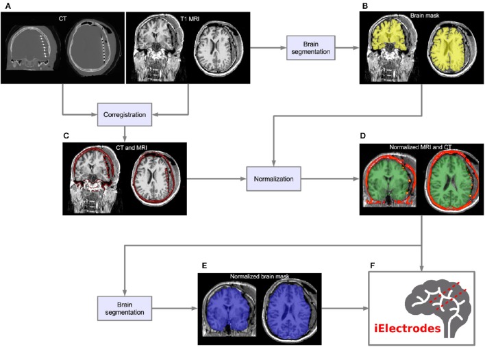
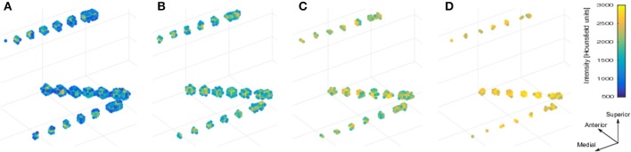
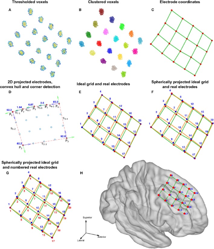
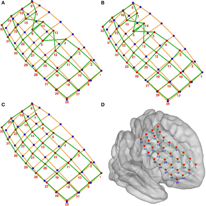
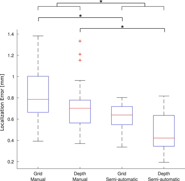
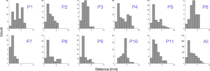
The localization of intracranial electrodes is a fundamental step in the analysis of invasive electroencephalography (EEG) recordings in research and clinical practice. The conclusions reached from the analysis of these recordings rely on the accuracy of electrode localization in relationship to brain anatomy. However, currently available techniques for localizing electrodes from magnetic resonance (MR) and/or computerized tomography (CT) images are time consuming and/or limited to particular electrode types or shapes. Here we present iElectrodes, an open-source toolbox that provides robust and accurate semi-automatic localization of both subdural grids and depth electrodes. Using pre- and post-implantation images, the method takes 2-3 min to localize the coordinates in each electrode array and automatically number the electrodes. The proposed pre-processing pipeline allows one to work in a normalized space and to automatically obtain anatomical labels of the localized electrodes without neuroimaging experts. We validated the method with data from 22 patients implanted with a total of 1,242 electrodes. We show that localization distances were within 0.56 mm of those achieved by experienced manual evaluators. iElectrodes provided additional advantages in terms of robustness (even with severe perioperative cerebral distortions), speed (less than half the operator time compared to expert manual localization), simplicity, utility across multiple electrode types (surface and depth electrodes) and all brain regions.

Keywords: CT; ECoG; MRI; SEEG; atlas; epilepsy; intracranial EEG.

Figure 1

Pre-processing pipeline. (A) Acquired images, CT and T1 MRI, showing electrode artifacts, brain shift and compression caused by edema. (B) A brain mask (yellow) is obtained by segmenting the MRI. Notice that the mask border follows the brain surface accurately. (C) MRI and CT images are coregistered in native space. Observe the electrode artifacts in the thresholded CT (red) over the MRI. (D) Using the previous brain mask (yellow), the MRI is spatially normalized and the same transformation applied to the CT. Observe the CT (red) on top of the normalized brain MRI. For illustrative purposes we also show the MNI average brain mask (green). (E) A normalized brain mask is obtained (blue) from the normalized MRI. (F) Normalized MRI, CT, and brain mask images are loaded into the iElectrodes toolbox. Example images correspond to patient 2, implanted with an 8 × 8 grid over the left frontal, temporal, and parietal lobes.

Figure 2

Voxels thresholding. The use of different threshold values on the CT produces more diffuse or clear views of the electrodes. (A) A low threshold value (700 HU) resulted in electrodes appearing to be merged together. (B,C) Middle threshold values (1,200 HU and 1,700 HU) resulted in a cleaner distinction between electrodes. (D) A high threshold value (2,200 HU) resulted in a few voxels per electrode. Notice that the two medial (deeper) contacts in each array are closer (3 mm) than all other contacts, making its visual differentiation more difficult. Example data from patient 17 showing one frontal and two temporal depth electrode arrays. HU, Hounsfield Units.

Figure 3

Localization and numbering of electrodes. (A) Thresholded CT voxels corresponding to a 4 × 5 grid (color coded HU) from patient 6. (B) Clustered voxels (each color denotes a different cluster). (C) Detected electrodes locations (red dots), i.e., center of mass of each cluster. (D) Electrode coordinates projected in 2D principal components space (blue circles). Convex hull described by a subset of points P (red asterisks) and segments S (red lines) connecting this points. Arrows show previous (green) and next (blue) segment direction at each point. The transition angle (in degrees) at each point is shown (blue). Points 1, 2, 3, and 4 correspond to the four biggest angles and also the corners of the grid. (E) Ideal planar grid (blue dots) and real grid electrode locations. Ideal grid electrodes are numbered (blue). (F) Radial projection of ideal electrode grids. (G) Real grid electrodes are numbered (red) according to closest ideal grid electrodes. (H) MNI semitransparent brain with localized and numbered electrodes.

Figure 4

Numbering of electrodes using permutation corrections. (A) First numbering of electrodes based on searching the minimum distance between ideal (blue dots) and real (red dots) electrodes. (B) Electrode numbering after first permutation correction. (C) Electrode numbering after second (last) permutation correction. (D) MNI semi-transparent brain with localized and numbered electrodes. Connecting lines are for illustrative purposes only. Example grid obtained from patient 3.

Figure 5

Localized electrodes in MRI-CT. MRI-CT blend images showing examples of electrode artifacts and detected coordinates (red crosses) superimposed. (A–C) Axial, sagittal and coronal views (respectively) of patient 6, implanted with a 4 × 5 grid over the right frontal lobe. (D) Sagittal view of patient 14 showing a depth electrode array in the insular cortex. (E,F) Coronal and sagittal view of patient 18 showing bilaterally implanted electrodes in hippocampi and temporal lobes.

Figure 6

Localized electrodes. (A) Summary plot of all grid and strip electrodes projected over the brain surface in MNI space. (B) Summary plot of all depth electrodes are shown in the MNI semi-transparent brain. Only half of the brain surface and corresponding electrodes are shown in each view (Superior: z > 0, Inferior: z < 0, Left: x < 0, Right x > 0, Anterior: y > 0, Posterior: y < 0).

Figure 7

Localization of electrodes in 3D view. (A) An example of localized of depth electrodes in a simple scenario, consisting of eight depth electrode arrays (Patient 22). (B) Example of localized of depth and grid electrodes in a complex scenario, formed by two grids and three depth electrode arrays entering through the gap between these two (Patient 5). In the last scenario, the selection of voxels in a 3D view is extremely simpler than the selection in 2D views. Additionally, the 3D view of localized coordinates on a rendered semitransparent brain helps to easily understand the relationship between electrodes and brain anatomy.

Figure 8

Localization error. Each boxplot shows the error (distance to the gold standard) for manual localization and for using iElectrodes to semiautomatically localize grids and depth electrodes. The center lines of each boxplot represents the median and the edges are the 25th (Q1) and 75th (Q3) percentiles. Whiskers are located at Q1 −1.5(Q3 −Q1) and Q3 +1.5(Q3 −Q1), and outliers are plotted outside this interval. ^*Denotes p < 1 × 10⁻⁵.

Figure 9

Distance to MNI cortex. Histograms showing the estimated distance of subdural grid electrodes to the smoothed cortical envelope (SCE) for each patient, P1–P11, and for all of them together.

References

1. Arnulfo G., Narizzano M., Cardinale F., Fato M. M., Palva J. M. (2015). Automatic segmentation of deep intracerebral electrodes in computed tomography scans. BMC Bioinformatics 16:99. 10.1186/s12859-015-0511-6 - DOI - PMC - PubMed
1. Ashburner J. (2007). A fast diffeomorphic image registration algorithm. Neuroimage 38, 95–113. 10.1016/j.neuroimage.2007.07.007 - DOI - PubMed
1. Ashburner J., Friston K. J. (1999). Nonlinear spatial normalization using basis functions. Hum. Brain Mapp. 7, 254–266. - PMC - PubMed
1. Avants B. B., Tustison N. J., Stauffer M., Song G., Wu B., Gee J. C. (2014). The Insight ToolKit image registration framework. Front. Neuroinform. 8:44. 10.3389/fninf.2014.00044 - DOI - PMC - PubMed
1. Axmacher N., Cohen M. X., Fell J., Haupt S., Dümpelmann M., Elger C. E., et al. (2010). Intracranial EEG correlates of expectancy and memory formation in the human hippocampus and nucleus accumbens. Neuron 65, 541–549. 10.1016/j.neuron.2010.02.006 - DOI - PubMed