Perceptual integration without conscious access

Abstract

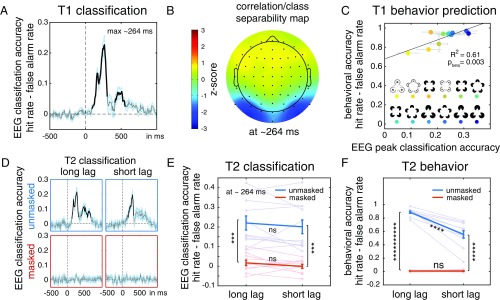
The visual system has the remarkable ability to integrate fragmentary visual input into a perceptually organized collection of surfaces and objects, a process we refer to as perceptual integration. Despite a long tradition of perception research, it is not known whether access to consciousness is required to complete perceptual integration. To investigate this question, we manipulated access to consciousness using the attentional blink. We show that, behaviorally, the attentional blink impairs conscious decisions about the presence of integrated surface structure from fragmented input. However, despite conscious access being impaired, the ability to decode the presence of integrated percepts remains intact, as shown through multivariate classification analyses of electroencephalogram (EEG) data. In contrast, when disrupting perception through masking, decisions about integrated percepts and decoding of integrated percepts are impaired in tandem, while leaving feedforward representations intact. Together, these data show that access consciousness and perceptual integration can be dissociated.

Keywords: access consciousness; attentional blink; masking; perceptual integration; phenomenal consciousness.

Fig. 1.

Experimental design. (A) Examples of different Kanizsa images and their controls as used in the experiment (Fig. S1 for the complete stimulus set). (B) Examples of two of the four trial types in the factorial design: without an AB (long lag) and strong masking (Left) and with an AB (short lag) and no masking (Right).

Fig. S1.

The 12 Kanizsa–control pairs; see SI Methods for rationale behind stimulus design.

Fig. S2.

Masks used during the experimental tasks. Triangular (A), square (B), pentagonal (C), and examples of lower-contrast nonmasks (D).

Fig. S3.

Independent RSVP task that was used to train the EEG classifier. Subjects were required to press a button whenever a black target would repeat (regardless of whether this target contained a Kanizsa or not), while ignoring the red distractors. Note that this task allowed us to train the classifier using a signal that was not contaminated by response mechanisms, decision mechanisms, or task relevance. We also performed an analysis in which these mechanisms were able to contribute, by training on T1 (Fig. 5).

Fig. 2.

Peak classification accuracy reflects perceptual integration. (A) T1 EEG mean decoding accuracy of perceptual integration over time. Line graphs are average ± SEM in light blue; thick black lines reflect P < 0.05, cluster-based permutation test. (B) The correlation/class separability map reflecting the underlying neural sources for maximum decoding at ∼264 ms (SI Methods). (C) The degree to which classification accuracy at ∼264 ms predicts behavioral sensitivity to perceptual integration at T1 for the 12 Kanizsa–control pairs when performing robust linear regression. Each colored data point is a Kanizsa–control pair (only the Kanizsa is shown in this figure; Fig. S1 for the full figure legend including the control counterparts). (D) T2 EEG decoding accuracy over time for the four experimental conditions and (E) maximum decoding accuracy at ∼264 ms for these conditions. (F) Behavioral sensitivity to perceptual integration for the four conditions (compare with E). Error bars are mean ± SEM; individual data points are plotted using low contrast in the background. ns, not significant (P > 0.05). ***P < 0.001, ****P < 10^–4, *****P < 10^–5, **********P < 10^–12.

Fig. S4.

Classifier weights when training on the 1-back RSVP task (A, Left) and the correlation class separability map (A, Right) at 264 ms. Line graphs are average ± SEM in light blue; thick black lines reflect P < 0.05, cluster-based permutation test. Because the signal is clearly occipital in nature, we compared T1 classification accuracy for all electrodes (B, Left) to classification accuracy for only the occipital electrodes (B, Right) PO7, PO3, O1, Iz, Oz, POz, PO8, PO4, O2; black dots in the topographic maps. Because the occipital electrodes result in superior performance, we used the occipital electrodes for the initial analyses (Figs. 2–4). Note, however, that using all electrodes and training on T1 (as in Fig. 5) did not substantially change the pattern of results.

Fig. S5.

Prediction of behavioral accuracy based on classifier performance in each of the four experimental conditions. (A) Behavioral accuracy within conditions based on classifier accuracy within those conditions. In both unmasked conditions, classification accuracy nicely predicts behavioral performance across the 12 Kanizsa–control pairs, albeit weaker in the short-lag AB condition. This is not surprising, given that access mechanisms are likely to dilute behavioral performance. (B) When using classifier performance to predict the uncontaminated T1 behavior, performance is invariably high in the unmasked conditions.

Fig. S6.

Contribution of frontal electrodes to perceptual integration. Although the signal related to perceptual integration is clearly occipital in nature (Fig. S4), a control analysis was performed to determine whether frontal electrodes contribute to this signal. (A) Classification accuracy for the four experimental conditions as well as T1, using only frontal electrodes: Fp1, AF7, AF3, Fpz, Fp2, AF8, AF4, AFz, and Fz. Right Bottom shows the topographic correlation/class separability map when using all electrodes (see SI Methods for details), with the frontal electrodes highlighted using black dots. (B) The degree to which this signal predicts behavioral performance across the 12 Kanizsa–control pairs in the four experimental conditions as well as T1. The frontal signal is invariably unable to predict behavioral performance across the 12 Kanizsa–control pairs (Fig. 2C and Fig. S5).

Fig. S7.

Seen–unseen analysis. (A) Splitting the main experiment up according to behavioral decision. (B) Splitting the masking control experiment up according to behavioral decision. Please read SI Results, Seen–Unseen Analysis, for an explanation of the pitfalls associated with behavior contingent selection of neural data and proper interpretation. Results are consistent with the main text.

Fig. 3.

Separating out perceptual integration and feature contrast detection. (A) Example stimuli that were used to orthogonally classify feature contrast and perceptual integration on the same data. (B) Classification accuracies across time for contrast detection and perceptual integration (Left) as well as correlation/class separability maps (Right) for T1, (C) and for unmasked (Left) and strongly masked trials (Right). Line graphs contain mean ± SEM. Thick lines are P < 0.05, cluster-based permutation test.

Fig. S8.

Contrast detection vs. perceptual integration. Stimuli used in the masking control analysis belonging to Fig. 3. Stimulus design was such that one could compare either in the contrast dimension or in the perceptual integration dimension, while collapsing orthogonally over the other dimension.

Fig. 4.

Masking control experiment. (A) Behavioral results. (B) Maximum classification accuracy. Error bars are mean ± SEM; individual data points are plotted in light in the background. *P < 0.05, ***P < 0.001. (C) Raw decoding accuracies over time for unmasked and weakly masked conditions. Line graphs contain mean ± SEM; black line reflects P < 0.05, cluster-based permutation test.

Fig. 5.

The impact of masking and AB on perceptual integration over time. (A) EEG classification accuracy for the four experimental T2 conditions when training on T1. (B) EEG classification accuracies and correlation/class separability maps plotted at peak classification performance at 264 ms (Top) and at the second peak at 406 ms (Bottom). Blue lines represent the unmasked condition; red lines represent the masked condition. The 406-ms time point follows the same pattern as behavioral accuracy (see main text for statistics) and has a spatial distribution that is homologous to that of a classical P300. ns, not significant (P > 0.05). *P < 0.05, **P < 0.01, ***P < 0.001, ****P < 10^–4, *****P < 10^–5, ******P < 10^–6. (C) An estimation of the GOF when using the normalized EEG classification accuracy data as a model for the normalized behavioral detection data (left axis). Datasets are either collapsed over the AB dimension (GOF masking), over the masking dimension (GOF AB), or without collapsing over either dimension (GOF masking, AB, and their interaction). T1 classification accuracy is plotted as a green shade in the background for reference (right axis). Not until after the perceptual integration signal has peaked at 264 ms does the black line overtake the red line, showing a postperceptual contribution of the AB to behavioral accuracy.

Fig. S9.

Classification accuracy for all electrodes and occipital electrodes when training and testing on T1 (eightfold leave-one-out procedure). Line graphs are average ± SEM in light blue; thick black lines reflect P < 0.05, cluster-based permutation test. Given the contribution of response and decision mechanisms to the response, we now see a slight enhancement when using all electrodes compared with when using occipital electrodes only (Fig. S4). Bottom panels shows graphs for the normalized responses when training on T1 at 264 and 406 ms, and normalized responses obtained from behavior. ns, not significant (P > 0.05). *P < 0.05, **P < 0.01, ***P < 0.001, ****P < 10^\x{2212}4, *****P < 10^–5, ******P < 10^–6, **********P < 10^–12.

References

1. Helmholtz HV. Handbuch der Physiologischen Optik. Leopold Voss, Leipzig; Germany: 1867.
1. Block N. Two neural correlates of consciousness. Trends Cogn Sci. 2005;9(2):46–52. - PubMed
1. Lamme VAF. How neuroscience will change our view on consciousness. Cogn Neurosci. 2010;1(3):204–220. - PubMed
1. Dehaene S, Changeux JP, Naccache L, Sackur J, Sergent C. Conscious, preconscious, and subliminal processing: A testable taxonomy. Trends Cogn Sci. 2006;10(5):204–211. - PubMed
1. Baars BJ. Global workspace theory of consciousness: Toward a cognitive neuroscience of human experience. Prog Brain Res. 2005;150:45–53. - PubMed
LinkOut - more resources