The Computational and Neural Basis of Rhythmic Timing in Medial Premotor Cortex

Abstract

The neural underpinnings of rhythmic behavior, including music and dance, have been studied using the synchronization-continuation task (SCT), where subjects initially tap in synchrony with an isochronous metronome and then keep tapping at a similar rate via an internal beat mechanism. Here, we provide behavioral and neural evidence that supports a resetting drift-diffusion model (DDM) during SCT. Behaviorally, we show the model replicates the linear relation between the mean and standard-deviation of the intervals produced by monkeys in SCT. We then show that neural populations in the medial premotor cortex (MPC) contain an accurate trial-by-trial representation of elapsed-time between taps. Interestingly, the autocorrelation structure of the elapsed-time representation is consistent with a DDM. These results indicate that MPC has an orderly representation of time with features characteristic of concatenated DDMs and that this population signal can be used to orchestrate the rhythmic structure of the internally timed elements of SCT.SIGNIFICANCE STATEMENT The present study used behavioral data, ensemble recordings from medial premotor cortex (MPC) in macaque monkeys, and computational modeling, to establish evidence in favor of a class of drift-diffusion models of rhythmic timing during a synchronization-continuation tapping task (SCT). The linear relation between the mean and standard-deviation of the intervals produced by monkeys in SCT is replicated by the model. Populations of MPC cells faithfully represent the elapsed time between taps, and there is significant trial-by-trial relation between decoded times and the timing behavior of the monkeys. Notably, the neural decoding properties, including its autocorrelation structure are consistent with a set of drift-diffusion models that are arranged sequentially and that are resetting in each SCT tap.

Keywords: drift-diffusion model; ensemble recordings; monkey; supplementary motor cortex; timing.

Figure 1.

A drift-diffusion model explains the rhythmic timing behavior of the monkeys. A, SCT. Monkeys were required to push a button (Responses, black line) each time stimuli with a constant interstimulus interval (stimuli, gray line) were presented, which resulted in a stimulus–movement cycle. After four consecutive synchronized movements, the stimuli stopped, and the monkeys continued tapping with a similar interval for three additional intervals. The instructed intervals, defined by brief auditory or visual stimuli, were 450, 550, 650, 850, and 1000 ms, and were chosen pseudorandomly within a repetition. B, Constant error (produced-instructed interval) of the animals during synchronization (blue) and continuation (red) phases of SCT as a function of the instructed duration. Monkeys slightly underestimated the interval durations during the continuation. C, The temporal variability of the monkeys increased as a function of instructed interval during both phases of SCT, with a larger slope in the continuation condition. D, Example diffusion trajectories for two different durations (450 and 850 ms) and on top the resulting distributions of produced intervals. E, Relationship between mean and SD of the produced interval of a DDM (red line) that is compared with the monkey's behavior during the continuation phase of the SCT (black line).

Figure 2.

SRTT. Monkeys required to push a button each time a stimulus was presented, but in this case the interstimulus interval was random (600–1400 ms), precluding the explicit temporalization of motor responses. Five stimulus–response cycles were collected in a sequence. Monkeys received a reward if the response time to each of five stimuli was within a 200–1000 ms window.

Figure 3.

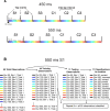
Illustration of the decoding analysis. A, Each trial consisted of six produced inter-tap intervals (S1–C3). Monkeys performed five trials in each of five instructed durations. To decode elapsed time during the inter-tap interval, we divided each interval into 50 ms bins. This meant that if the monkey produced a perfect instructed 550 interval, the total number of bins for this interval would be 11 (550/50 = 11). We then calculated the discharge rate for the cells recorded simultaneously in a session within each 50 ms bin of a produced interval, keeping this information independently for each of the six serially produced intervals, and each of the five instructed intervals. Thus, we organized the neural data for each bin and trial into observations. The total number of observations corresponded to the total number of bins defined by the duration of the produced intervals by the monkey during the five trial repetitions. B, For a perfect execution across trials for the interval of 550 ms, the total number of observations correspond to 55 (11 bins × 5 repetitions). We determined the degree to which neural activity represented the passage of time by classifying each observation as one of the n time bins produced by the monkey, based on the pattern of firing rates across the population of cells. In this analysis, 4/5 of the observations were used as training data to obtain an average pattern of activity across the neural population for each time bin. The activity pattern recorded on each of the remaining 1/5 of observations were used as the testing observations, and were compared with the average patterns. The result of this comparison was the classification of each testing observation as the time bin with the closest matching average pattern. This process was repeated four more times, namely, the bins of all the repetitions were used as testing observations. Consequently, all the classified bins were kept as decoded durations associated to a true bin in a produced interval.

Figure 4.

Comparison between the produced intervals by the monkey and the DDM model. A, Distribution of the produced intervals by the two monkeys for the five instructed intervals (red line) and the corresponding distribution of time estimates by the DDM (blue line). B, Coefficient of variation (CV) as a function of the instructed intervals of the monkeys' produced intervals. C, Skew of the distributions in A of the produced intervals by the monkeys as a function of the instructed intervals. D, Skew to CV ratio of the distributions in A produced intervals by the monkeys as a function of the instructed intervals.

Figure 5.

Average spike density functions (spikes/s, σ = 30 ms) of single cells responding after the button press (time 0 ms in the abscissas) across instructed intervals in the SCT. A, Neuronal activity of a cell whose activity increases linearly with elapsed time for all instructed intervals. B, Neuronal activity of a cell that shows a duration increase in its up–down activation profile as a function of instructed interval. C, Activity of a cell that shows an increase in discharge rate across target intervals; however, there is also an asymptotic saturation of the response linked to the instructed interval. The color code for target intervals is described in B (inset). Note that different nonlinear patterns of ramping activity modulated by the instructed intervals are present in our database. From 475 neurons used for the decoding of Figure 7, 240 neurons showed ramping activity whose duration, peak activity, and/or slope showed significant differences for instructed interval (ANOVA, p < 0.05).

Figure 6.

Time decoding based on individual serial order elements is more robust than using all the sequence of the SCT. A, Number of recording sessions that showed significant linear relations between the decoded and actual time bins across the five instructed intervals and the six serial-order elements of the SCT. Each of the 53 recording sessions could add a maximum of 30 counts in the plot (5 instructed intervals by 6 serial-order elements) if the decoded values for each interval/serial-order combination showed a significant relation between the decoded and the elapsed time. Note that all the combinations of instructed intervals and serial-order elements are represented in the population decoding. B, The entropy for individual serial-order elements is smaller than the entropy of the decoding posterior probabilities using all serial-order, indicating that the different cell populations carry duration information for specific serial-order elements.

Figure 7.

Time decoding during the SCT. A, Median (black dot) and interquartile (blue bar) values of the decoded times as a function of instructed time for the 1000 ms interval. The blue dots correspond to outlier data. B, Bimodal distribution of the decoded times of the first bin (50 ms) in B, where the bimodal mixture model converged with a low (red) and a high value mode (blue). C, Unimodal distribution the decoded times of the bin 10 (500 ms) in B. The mean is close to the target bin time. D–H, Mean ± STD (across recording sessions and 3 serial-order elements) for the unimodal (only red dots in the intermediate bins) and the bimodal mixture (red and blue circles in the extreme bins of the interval) models for the five instructed intervals of the continuation phase. The number of blue dots in each instructed interval depended on the significance of the bimodal model in each time bin. I, Mean (±SEM) of the second μ of bimodal mixture for the earlier bins (μ-previous) and the last bins (μ-next) as a function of the instructed time. Note how the μ-previous scales with the duration of the instructed interval. J, The animals' interval error (produced-instructed interval) as a function of the six serial-order elements of the task, three in the synchronization (S1–S3) and three in the continuation (C1–C3) phase, for the first four bins of the 1000 ms instructed interval. The behavior was divided on the trials associated with the larger (blue) and smaller (red) mode of the decoding times in H. K, Same as J but for the last four bins of the 1000 ms instructed interval. In this case, the behavior was divided on the trials associated with the smaller (blue) and larger (red) mode of the decoding times in H.

Figure 8.

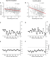
Trial-by-trial relation between decoding and behavior. A, B, Negative correlation between the error in decoded time and the animals' time error on a trial-by-trial basis. There is a larger significant negative correlation between these two measures in the continuation (B) than the synchronization phase (A). C, D, Percentage of significant negative correlations (from 15 conditions that come from 5 instructed intervals and 3 serial order elements) between the decoded and the behavioral error as a function of the time to the next tap, for the synchronization (C) and continuation (D) conditions. E, F, Pearson correlation coefficient (r) for significant (p < 0.05) negative correlations between the decoded and the behavioral error as a function of the time to the next tap, for the synchronization (E) continuation (F) conditions.

Figure 9.

Similar autocorrelation structure between the decoding data and the DDM. A, B, Autocorrelation matrix of the decoded times for the 850 ms instructed interval across time bins within produced intervals. During the continuation phase (B), the autocorrelation is broader than during the synchronization phase (A). C, Autocorrelation function for a diffusion process. D, Relationship between model estimate of autocorrelation and measured autocorrelation of the process in the decoded data (mean ± SEM).

Figure 10.

Comparing the decoding during the synchronization phase of the SCT and the SRTT. A, The mean ± STD for the unimodal distribution of decoded times during the SRTT control task shows a weak relation with the actual instructed time. In contrast, the decoded times linked to the actual time representation show a linear relation (slope = 0.943) with the instructed time during the 1000 ms interval of the synchronization phase of the SCT. In addition, the second mode of the bimodal mixture model (blue circles) is associated with the time bins of the previous and next serial-order elements of the SCT task during the extreme bins of the interval. B, Entropy of the decoding posterior probabilities for the synchronization phase of the SCT and the SRTT. C, Mean ± STD of the temporal variability (SD) of the decoded times across bins for the synchronization phase of the SCT and the SRTT.

Figure 11.

Autocorrelation matrix during 800 ms of activity of units in a recurrent artificial neural network that could reproduce sequential spatiotemporal patterns and the scalar property of interval timing (data kindly shared by Dean Buonomano from Laje et al., 2011, their Fig. 6B).

References

1. Bakhurin KI, Goudar V, Shobe JL, Claar LD, Buonomano DV, Masmanidis SC (2017) Differential encoding of time by prefrontal and striatal network dynamics. J Neurosci 37:854–870. 10.1523/JNEUROSCI.1789-16.2017 - DOI - PMC - PubMed
1. Buonomano DV. (2000) Decoding temporal information: a model based on short-term synaptic plasticity. J Neurosci 20:1129–1141. - PMC - PubMed
1. Churchland AK, Kiani R, Chaudhuri R, Wang XJ, Pouget A, Shadlen MN (2011) Variance as a signature of neural computations during decision making. Neuron 69:818–831. 10.1016/j.neuron.2010.12.037 - DOI - PMC - PubMed
1. Crowe DA, Zarco W, Bartolo R, Merchant H (2014) Dynamic representation of the temporal and sequential structure of rhythmic movements in the primate medial premotor cortex. J Neurosci 34:11972–11983. 10.1523/JNEUROSCI.2177-14.2014 - DOI - PMC - PubMed
1. Gibbon J. (1977) Scalar expectancy theory and Weber's law in animal timing. Psychol Rev 84:279–325. 10.1037/0033-295X.84.3.279 - DOI
Publication types
LinkOut - more resources