The evolution of postpairing male mate choice

Abstract

An increasing number of empirical studies in animals have demonstrated male mate choice. However, little is known about the evolution of postpairing male choice, specifically which occurs by differential allocation of male parental care in response to female signals. We use a population genetic model to examine whether such postpairing male mate choice can evolve when males face a trade-off between parental care and extra-pair copulations (EPCs). Specifically, we assume that males allocate more effort to providing parental care when mated to preferred (signaling) females, but they are then unable to allocate additional effort to seek EPCs. We find that both male preference and female signaling can evolve in this situation, under certain conditions. First, this evolution requires a relatively large difference in parental investment between males mated to preferred versus nonpreferred females. Second, whether male choice and female signaling alleles become fixed in a population versus cycle in their frequencies depends on the additional fecundity benefits from EPCs that are gained by choosy males. Third, less costly female signals enable both signaling and choice alleles to evolve under more relaxed conditions. Our results also provide a new insight into the evolution of sexual conflict over parental care.

Keywords: Extra-pair copulation; female sexual signal; male mate choice; parental care; postpairing.

Figure 1

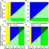
The conditions required for local stability of the four cases of fixation of alleles at the P or S loci, and the existence of an internal equilibrium. Regions indicated in light green plus the medium‐green represent the conditions for the local stability of (0, 0, 0). Equilibrium (1, 0, 0) is stable in the left yellow region. The region indicated in medium‐green also represents the conditions required for the local stability of (1, 1, 0) and the existence of a unstable internal equilibrium. In this region, there is bistability, such that both (1, 1, 0) and (0, 0, 0) are stable equilibria. The regions with dark green in (A) and (C) represents the conditions for only one stable equilibrium (1, 1, 0). Regions indicated in blue represent the conditions required for the existence of cycling around the internal equilibrium. The vertical dashed line shows the threshold value of δ₁ when ${\delta }_2=\frac{(1+b)t-b{\delta }_1}{b(1-t)}$, the oblique dashed line is $d_{c1}=b{\delta }_1$. We set ${\delta }_2=0.2$ to enable $d_{c2}<b{\delta }_2(1-t)$ in (A) and (C), and ${\delta }_2=0.1$ to enable $d_{c2}>b{\delta }_2(1-t)$ in (B) and (D), The other parameters are: $b=0.8$, $c=1.0$, $d_{c2}=0.1$; $t=0.2$ in (A) and (B), and $t=0.1$ in (C) and (D).

Figure 2

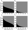
Numerical results of the bistable system with different initial frequencies of $(p_2,s_2,0)$, ranging from 0.0 to 1.0 with a step size of 0.01. Regions indicated in black represent the population that will achieve the equilibrium of (0, 0, 0) from the corresponding initial state. Regions indicated in gray represent the population that will achieve the equilibrium of (1, 1, 0). There are two red dots representing the equilibria (1, 0, 0) and (0, 1, 0). The other parameters are: $b=0.8$, $r=0.5$, $c=0.9$, ${\delta }_1=0.3$, ${\delta }_2=0.35$; $t=0.1$ in (A) and (C) and $t=0.01$ in (B) and (D); $d_{\mathrm{c}1}=0.2$, $d_{\mathrm{c}2}=0.23$ in (A) and (B), and $d_{\mathrm{c}1}=0.15$, $d_{\mathrm{c}2}=0.2$ in (C) and (D).

Figure 3

Frequency dynamics of two alleles under different initial frequencies when the internal equilibrium exists. Simulations are ran for a total of 15,000 generations. The initial state is set to (0.1, 0.1, 0) in (A) and (C), and (0.5, 0.5, 0) in (B) and (D). The points shown in (A) and (B) are the corresponding internal equilibrium of the model. (C, D) The frequency dynamics of the alleles P₂ (red curve) and S₂ (green curve) during the last 1000 generations of (A) and (B), respectively. The other parameters are: $b=0.8$, $t=0.1$, $c=0.9$, $d_{\mathrm{c}1}=0.8$, $d_{\mathrm{c}2}=0.75$, $r=0.001$, and ${\delta }_1=0.2$, ${\delta }_2=0.25$.

Figure 4

Frequency dynamics of two alleles and linkage disequilibrium under different recombination rates when the internal equilibrium exists. The red curve in the above figures represents the frequency of P₂ and the green curve the frequency of S₂. The initial state is set to (0.5, 0.5, 0). (A)$r=0.5$, (B) $r=0.1$, and (C) $r=0.001$. The other parameters are the same as in Figure 3.

Figure 5

Representative figures of the relative importance of unequal changes in male parental care (i.e., δ₁ and δ₂) and potential extra‐pair benefits and costs (i.e., $d_{c1}$ and $d_{c2}$). In (A) and (B), we set $d_{c1}=d_{c2}=d_c$ and ${\delta }_1=\alpha {\delta }_2$ to assess the relative effect of the reduction (δ₁, when P₂ males mate with S₁ females) versus increase (δ₂, when P₂ males mate with S₂ females) in parental care. In (C) and (D), we set ${\delta }_1={\delta }_2=\delta$ and $d_{c1}=\beta d_{c2}$ to assess the relative effect of the increase ($d_{c1}$, when P₂ males mate with S₁ females) versus reduction ($d_{c2}$, when P₂ males mate with S₂ females) in extra‐pair mating benefits. The color definitions for local stabilities are generally the same as in Figure 1. The regions with dark green in (B–D) represents the conditions for only one stable equilibrium of (1, 1, 0). In (A) and (B), the oblique dashed line is $d_c=b{\delta }_1$, the horizontal gray dashed line is $d_c=b{\delta }_2(1-t)$, the vertical black dashed line shows $\alpha =1-t$, and the gray dashed line represents the corresponding value of α when ${\delta }_2=\frac{(1+b)t-b{\delta }_1}{b(1-t)}$. In (C) and (D), the oblique dashed line shows $d_{c1}=b\delta$, the vertical black dashed line shows $d_{c2}=b\delta (1-t)$ and the gray one represents $\delta =\frac{(1+b)t}{b(2-t)}$. We set ${\delta }_2=0.2$ in (A) and (B) and $d_{c2}=0.5$ in (C) and (D) for illustration. The other parameters are: $b=0.9$, $c=1.0$, $t=0.2$ in (A) and (C), and $t=0.1$ in (B) and (D).

Figure 6

Schematic of the allele frequency oscillations when an internal equilibrium exists in the model.

References

1. Amundsen, T. 2000. Why are female birds ornamented? Trends Ecol. Evol. 15:149–155. - PubMed
1. Amundsen, T. , and Forsgren E.. 2001. Male mate choice selects for female coloration in a fish. Proc. Natl. Acad. Sci. U. S. A. 98:13155–13160. - PMC - PubMed
1. Andersson, M.B. 1994. Sexual selection. Princeton Univ. Press, Princeton, NJ.
1. Barry, K. L. , and Kokko H.. 2010. Male mate choice: why sequential choice can make its evolution difficult. Anim. Behav. 80:163–169.
1. Berzins L. L., and Dawson R. D.. 2016. Experimentally altered plumage brightness of female tree swallows: a test of the differential allocation hypothesis. Behaviour 153:525–550.