Image analysis driven single-cell analytics for systems microbiology

Abstract

Background: Time-lapse microscopy is an essential tool for capturing and correlating bacterial morphology and gene expression dynamics at single-cell resolution. However state-of-the-art computational methods are limited in terms of the complexity of cell movies that they can analyze and lack of automation. The proposed Bacterial image analysis driven Single Cell Analytics (BaSCA) computational pipeline addresses these limitations thus enabling high throughput systems microbiology.

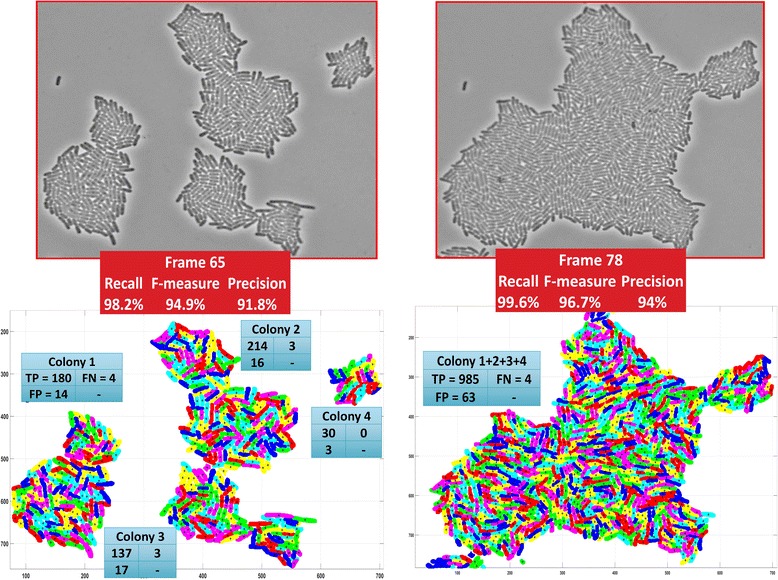
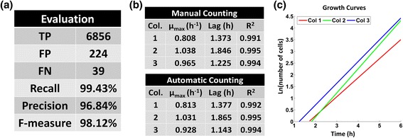
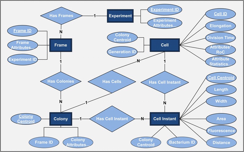
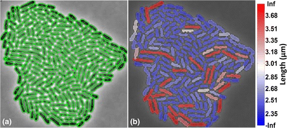
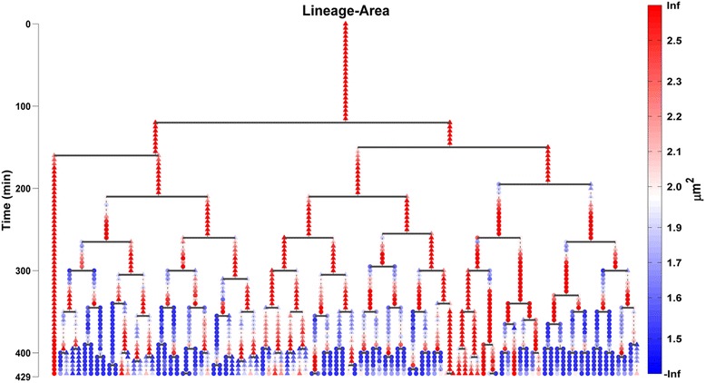
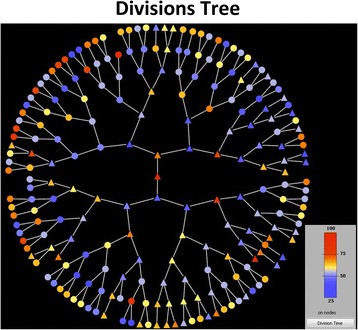
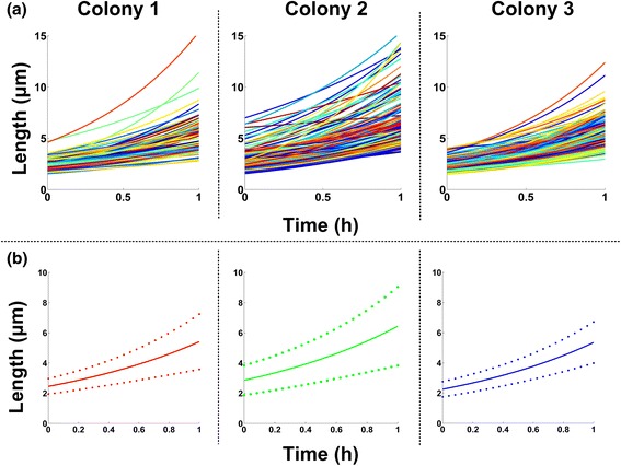
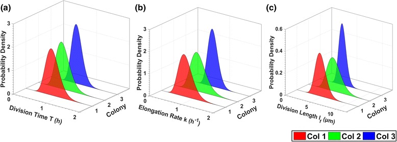
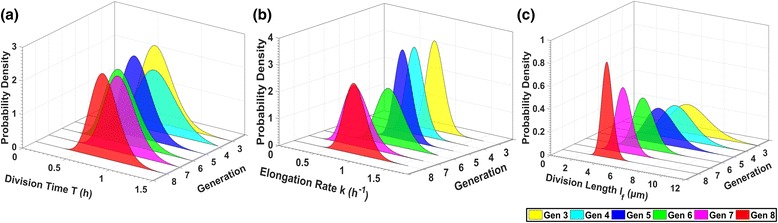
Results: BaSCA can segment and track multiple bacterial colonies and single-cells, as they grow and divide over time (cell segmentation and lineage tree construction) to give rise to dense communities with thousands of interacting cells in the field of view. It combines advanced image processing and machine learning methods to deliver very accurate bacterial cell segmentation and tracking (F-measure over 95%) even when processing images of imperfect quality with several overcrowded colonies in the field of view. In addition, BaSCA extracts on the fly a plethora of single-cell properties, which get organized into a database summarizing the analysis of the cell movie. We present alternative ways to analyze and visually explore the spatiotemporal evolution of single-cell properties in order to understand trends and epigenetic effects across cell generations. The robustness of BaSCA is demonstrated across different imaging modalities and microscopy types.

Conclusions: BaSCA can be used to analyze accurately and efficiently cell movies both at a high resolution (single-cell level) and at a large scale (communities with many dense colonies) as needed to shed light on e.g. how bacterial community effects and epigenetic information transfer play a role on important phenomena for human health, such as biofilm formation, persisters' emergence etc. Moreover, it enables studying the role of single-cell stochasticity without losing sight of community effects that may drive it.

Keywords: Bacterial image analysis; Cell segmentation; Colonies segmentation; Lineage tree construction; Machine learning; Single-cell analytics; Single-cell informatics; Time-lapse microscopy; Visualization.

Fig. 1

Image preprocessing and Colonies Segmentation. a Input image with three colonies (SalPhase movie). b Contourlet based denoising and adaptive histogram equalization used to sharpen cell edges. c Colony masks created using morphological filtering, Otsu’s global thresholding and Canny edge detection; they are used to separate colony regions from image background so that each colony can be processed separately in the pipeline (divide-and-conquer). d Adaptive thresholding is used to remove the colony’s local background pixels. e Multiplication of the image generated by adaptive thresholding with the corresponding extracted mask (Colony in the red rectangle) removes the noise (existing locally in the colony) and the artifacts (produced by the adaptive thresholding algorithm) while revealing cell objects inside the colony

Fig. 2

Overview of the cells segmentation method. (1) Colonies segmentation. (2) Objects identification inside a colony. (3) Skeleton based object classification; (4) Complex object segmentation: 4a) Watershed algorithm application, 4b) “puzzle solving” step, 4c) new dataset generation, 4d) unsupervised Gaussian mixture modeling, 4e) final result of bacterial cells segmentation. (5) Collinear object segmentation: 5a) Application of the “deep valley" criterion to identify “bow tie” points, 5b) final result of bacterial segmentation. At step (3), there is a bifurcation leading to different processing routes based on the object's classification. See text for details

Fig. 3

Cell Objects extraction and classification. a Each colony is an ensemble of cell objects corresponding to one or more “touching” cells; e.g. see three cell objects marked with color. We first extract the skeleton of each object and classify it as complex (red) or collinear (green) according to the presence (or absence) of skeleton junctions (i.e. skeleton pixels with more than two neighbors). b The skeleton of the smaller red object has two junctions (marked with yellow boxes) so it is classified as a complex object. c Colony object with no junctions (green) classified as collinear object. d A complex object (large red) with four junctions. See text for details

Fig. 4

Collinear objects analysis - "Bow ties" identification. a Extracted collinear object. b Skeletonized object with skeleton pixels numbered. The red numbers mark the “bow tie" locations on the centerline. c Distance curve of the object: To construct it we form pairs of opposite-side diametric boundary pixels (w.r.t. the skeleton) and compute their Euclidean distance (local width). Then we search for “deep valleys” (i.e. significant local minima relative to neighboring local maxima (marked with red circles for illustration purposes) and, (d) we split the object at bowtie points (marked by red dashed lines for illustration purposes), that correspond to the deep valley positions in (c). e The collinear object is segmented into three single-cells

Fig. 5

Distance transform. a Cell object depicted in 3D; the image pixel intensities are shown in the z-axis. b Same object's distance transform in 3D; the distance values are shown in the z-axis. It is obvious that the distance transform [40] smoothens object abnormalities while sharpening the valley between the two cells comprising the cell object

Fig. 6

Complex object Analysis - Generation of a dataset representing the object. a A very complex object (large number of cells) including potentially 75 single-cells. b Data points generation for the object in (a) by random sampling (see text for details), 9240 data points generated. c A less complex object with only 6 potential cells. d Data points generation for object in (c), 740 data points generated. The number of generated data points is proportional to the number of the complex object centroids, thus it depends on the object’s structural complexity (number of potential cells included). Also, more data points are randomly “thrown” around the cells’ medial axes, so as to best represent cell structures (see text for details)

Fig. 7

Cells segmentation - Best Gaussian Mixtures Model fit. Initialization of Gaussian mixture model parameters is performed after associating data points to cluster centers using nearest neighbor classification. For the complex object in (a) we have initially C = 6 components (clusters) in the mixture and for the model in (c) C = 17 components. We then apply the Expectation-Maximization (EM) algorithm and use the Minimum Message Length (MML) model selection criterion to identify the number of mixture model components that produces the best model fit. In (b) this results to a reduction of clusters from 6–4, and in (d) from 17–15. Each component in the final model represents a segmented single-cell (see text for details)

Fig. 8

Comparative Evaluation Summary. Each section of the table reports the evaluation results for an image suggested by one of the methods under comparison. The table columns list the true positives (TP), false positives (FP), false negatives (FN), as well as the Recall, Precision and F-measure achieved by each method. SalPhase frame 74 and Multi-SalPhase frame 78 were used to assess the performance of the methods on images with dense and overcrowded colonies. Dashes (-) indicate failure to return results for a specific dataset. Tildes (~) indicate very poor performance. The proposed method (BaSCA) achieved consistently very high F-measure (≥97.3% for all cases), suggesting that it is robust across imaging modalities and datasets produced by different labs. (Refer to Additional file 1: Figures S1-S5 for the detailed segmentation results)

Fig. 9

Segmentation of overcrowded and merging colonies. The four colonies in frame 65 of movie Multi-SalPhase (left) are merged several frames later (frame 78, right). Top panels: input image frames. Bottom panels: Segmentation results: The cyan boxes report the TP, FN and FP for each colony. The red boxes summarize the evaluation measures for each frame. Pseudo-colors are used to make cell boundaries visible. BaSCA achieves both high recall and high precision and an F-measure over 94%

Fig. 10

Growth rates - Evaluation w.r.t. the ground truth. a Evaluation results summary for the SalPhase movie (86 frames). The developed pipeline achieves a very high F-measure above 98%, (b) Comparison of manual vs. automatic BaSCA counting for the three colonies of the SalPhase movie by fitting a Baranyi and Roberts model [43]; the kinetic parameters of microbial growth are almost identical, (c) Automatically estimated growth curves of the three micro-colonies in the dataset

Fig. 11

Single-cell analytics database ER-Diagram. Organization of the database storing information about the experiment that generated the cell movie (Experiment table) and the time lapse microscopy characteristics (Frame table). In addition, we store the image analysis generated information for each colony in the field of view (Colony Table) and for each segmented cell within each colony. Specifically, single-cell attribute values changing at every time point are stored in the Cell Instant Table, while cell life attributes that characterize the whole cell life trajectory are stored in the Cell Table. The database summarizes the cell movie image analysis completely and can be used for downstream single-cell analytics and visualization. Moreover it forms the basis for building repositories of cell movies under different conditions for large scale high throughput systems microbiology experiments

Fig. 12

Cell attribute visualization. a BaSCA segmentation results for colony 3 of the SalPhase movie (frame 86). Green curvatures mark the contours of segmented cells. b Cell length visualization using color, overlaid on each segmented cell. Movies of cell length visualization are provided in Additional file 4 and 5 for SalPhase and Multi-SalPhase datasets respectively

Fig. 13

Single-cell attribute evolution visualization on the lineage tree. The lineage tree of colony 1 (top left) of the SalPhase movie. The area attribute is visualized using color on the tree for every cell and time instant (frame) of the movie. Triangular (circular) shape node glyphs are used for time instants that a cell lies in the colony’s boundary or within the colony respectively. Any cell attribute available in the database produced by the image analysis can be visualized in the same manner

Fig. 14

Cell life attribute visualization on the cell divisions tree. A circular tree of cell divisions (root cell in the middle) for colony 3 of the SalPhase cell movie. Colors represent here division times (min) as indicated by the color bar. We can easily assess visually how division times vary along tree branches (cell clones) and tree levels (cell generations). Triangular (circular) nodes represent cells that lie on the colony’s boundary (within the colony) respectively. Any cell life attribute available in the database produced by the image analysis can be visualized in the same manner. The Figure was created using the Tulip software package [67]

Fig. 15

Single-Cell Exponential Growth curves. a Single-cell growth curves estimated from the image-analysis data after fitting an exponential individual cell length model (see text for details). Different colors represent different single-cell lifespan trajectories. b Average cell growth curves of each colony (solid lines). Dashed lines represent one standard deviation above and below the average curve. We observe that cell growth exhibits considerable variability among colonies, and cells within the same colony (SalPhase cell movie)

Fig. 16

Life attributes variability per colony. Gamma distributions (best fit) of (a) the cell division time T, (b) the cell elongation rate k, (c) the cell division length l _f for colonies 1, 2 and 3 (SalPhase movie). The proposed methodology allows us to characterize the variability of cell life attributes across colonies. Similar analysis can be performed for any life attribute available in the database after image analysis using BaSCA

Fig. 17

Life attributes variability per generation. Gamma distributions (best fit) of (a) the cells division time T, (b) the cell elongation rate k, and (c) the cell length at division l _f for the 3^rd to the 8^th generation of cells of the SalPhase movie (cells from all colonies pooled). By delving into each generation’s individuals we can characterize a life attribute's intra and inter-generation variability (stochasticity). Similar analysis can be performed for any life attribute available in the database after image analysis using BaSCA

References

1. Korobkova E, Emonet T, Vilar JMG, Shimizu TS, Cluzel P. From molecular noise to behavioral variability in a single bacterium. Nature. 2004;428:574–578. doi: 10.1038/nature02404. - DOI - PubMed
1. Arias AM, Hayward P. Filtering transcriptional noise during development: concepts and mechanisms. Nat Rev Genet. 2006;7:34–44. doi: 10.1038/nrg1750. - DOI - PubMed
1. Avery SV. Microbial cell individuality and the underlying sources of heterogeneity. Nat Rev Microbiol. 2006;4:577–587. doi: 10.1038/nrmicro1460. - DOI - PubMed
1. Kaern M, Elston TC, Blake WJ, Collins JJ. Stochasticity in gene expression: from theories to phenotypes. Nat Rev Genet. 2005;6:451–464. doi: 10.1038/nrg1615. - DOI - PubMed
1. Raser JM, O’Shea EK. Noise in gene expression: origins, consequences, and control. Science. 2005;309:2010–2013. doi: 10.1126/science.1105891. - DOI - PMC - PubMed
Publication types
LinkOut - more resources