Neural coding of time-varying interaural time differences and time-varying amplitude in the inferior colliculus

Abstract

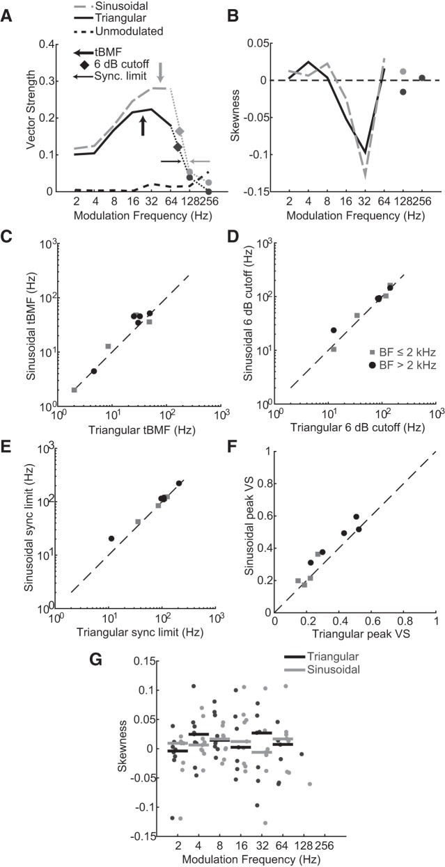
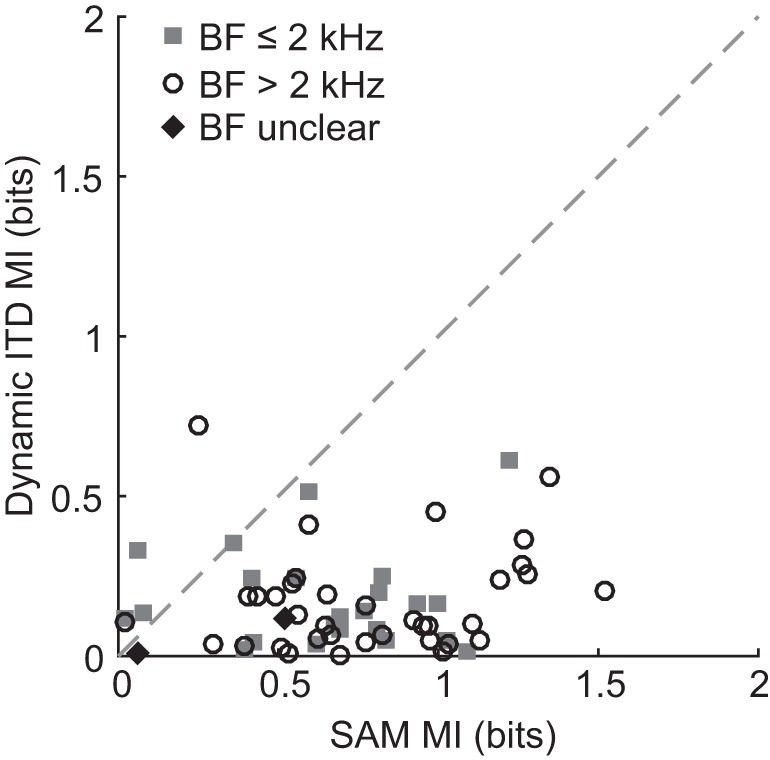
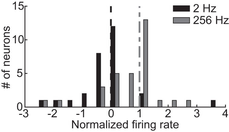
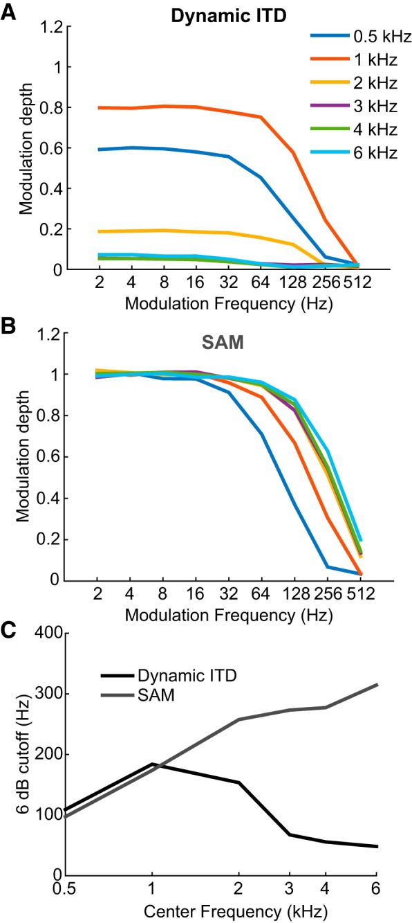
Binaural cues occurring in natural environments are frequently time varying, either from the motion of a sound source or through interactions between the cues produced by multiple sources. Yet, a broad understanding of how the auditory system processes dynamic binaural cues is still lacking. In the current study, we directly compared neural responses in the inferior colliculus (IC) of unanesthetized rabbits to broadband noise with time-varying interaural time differences (ITD) with responses to noise with sinusoidal amplitude modulation (SAM) over a wide range of modulation frequencies. On the basis of prior research, we hypothesized that the IC, one of the first stages to exhibit tuning of firing rate to modulation frequency, might use a common mechanism to encode time-varying information in general. Instead, we found weaker temporal coding for dynamic ITD compared with amplitude modulation and stronger effects of adaptation for amplitude modulation. The differences in temporal coding of dynamic ITD compared with SAM at the single-neuron level could be a neural correlate of "binaural sluggishness," the inability to perceive fluctuations in time-varying binaural cues at high modulation frequencies, for which a physiological explanation has so far remained elusive. At ITD-variation frequencies of 64 Hz and above, where a temporal code was less effective, noise with a dynamic ITD could still be distinguished from noise with a constant ITD through differences in average firing rate in many neurons, suggesting a frequency-dependent tradeoff between rate and temporal coding of time-varying binaural information.NEW & NOTEWORTHY Humans use time-varying binaural cues to parse auditory scenes comprising multiple sound sources and reverberation. However, the neural mechanisms for doing so are poorly understood. Our results demonstrate a potential neural correlate for the reduced detectability of fluctuations in time-varying binaural information at high speeds, as occurs in reverberation. The results also suggest that the neural mechanisms for processing time-varying binaural and monaural cues are largely distinct.

Keywords: amplitude modulation; auditory motion; binaural sluggishness; inferior colliculus; reverberation.

Fig. 1.

Running cross-correlation of the two channels for 1 s of a 4-Hz triangular dynamic ITD stimulus (A), a sinusoidal dynamic ITD stimulus (B), an Oscor stimulus (Joris et al. 2006) (C), and a phasewarp stimulus (Dietz et al. 2008; Siveke et al. 2008) (D) as a function of time. For the stimuli shown, the magnitude of the spectrum below 50 Hz and above 15 kHz was set to zero. Each cross-correlation was performed within 2-ms Hanning windows. Neighboring windows were half-overlapping.

Fig. 2.

A: creation of a time-varying interaural delay in a window of broadband noise. The original signal was zero-padded in the frequency domain to 10 times its original length, resulting in a 10× upsampled signal. The upsampled signal was then resampled with a time-varying delay. The original noise was presented through the contralateral channel, and the delayed noise was presented through the ipsilateral channel, resulting in a dynamic ITD. B: cross-correlation of a 4-Hz triangular dynamic ITD stimulus. This plot is identical to Fig. 1A.

Fig. 3.

A: static ITD tuning curve measured in an example neuron (BF = 3,512 Hz). The black arrow designates the ITD range of the dynamic ITD stimulus presented for this neuron. The gray arrow designates the ITD of the SAM stimulus. B: period histograms for the dynamic ITD and SAM for this neuron. C: tMTFs for SAM (gray) and dynamic ITD (black). The dotted lines connect to vector strengths that are not significant, indicated by circles (P > 0.001 by the Rayleigh test with Bonferroni correction). Thick arrows indicate the tBMFs, diamonds indicate the 6-dB cutoff, and thin arrows indicate the synchronization limits (sync. limit). For this neuron, all of the temporal metrics examined were higher for SAM than for dynamic ITD (sync. limit: SAM = 169 Hz, dynamic ITD = 82 Hz; peak VS: SAM = 0.81, dynamic ITD = 0.65; 6-dB cutoff: SAM = 56 Hz, dynamic ITD = 43 Hz; tBMF: SAM = 23 Hz, dynamic ITD = 11 Hz). D: mean phases for SAM (gray) and dynamic ITD (black) along with the linear fit (SAM: group delay = 20.1 ms, phase intercept = −0.28 cycles, R² = 0.98; dynamic ITD: group delay = 17.2 ms, shifted phase intercept = −0.06 cycles, R² = 0.98). Only phases where phase locking was significant are shown. E: rMTFs for SAM (gray) and dynamic ITD (black) with SE. The average rates to the unmodulated stimuli for both SAM and dynamic ITD are shown as dashed lines. For this neuron, the MI was higher for SAM than dynamic ITD (SAM: MI = 0.95; dynamic ITD: MI = 0.10). F: skewness as a function of modulation frequency for SAM (gray) and dynamic ITD (black). Skewness values at modulation frequencies with nonsignificant phase locking are labeled with circles.

Fig. 4.

Example low-BF neuron (BF = 842 Hz). Data in A–F are plotted as described for Fig. 3 (sync. limit: SAM was beyond measured values, dynamic ITD = 52 Hz; 6-dB cutoff: SAM = 184 Hz, dynamic ITD = 35 Hz; tBMF: SAM = 15 Hz, dynamic ITD = 14 Hz; peak VS: SAM = 0.42, dynamic ITD = 0.25; SAM: MI = 0.42, dynamic ITD: MI = 0.24; SAM: group delay = 11.5 ms, shifted phase intercept = −0.04 cycles, R² = 0.997; dynamic ITD: group delay = 20.5 ms, shifted phase intercept = −0.09 cycles, R² = 0.9996).

Fig. 5.

A: the fraction of neurons out of 66 with significant vector strengths at each modulation frequency for SAM (gray) and dynamic ITD (black). B: vector strength of all of the neurons measured (n = 66) for SAM and dynamic ITD at each modulation frequency. Horizontal bars indicate median values.

Fig. 6.

Comparison of SAM and dynamic ITD tBMFs (A), 6-dB cutoffs (B), synchronization limits (C), and peak vector strengths (D) in 62/66 neurons. All of these metrics were significantly higher for SAM than for dynamic ITD across the population (Wilcoxon signed-rank test: P < 0.001). In all of these plots, neurons with BF <2 kHz are represented by gray squares, neurons with BF >2 kHz are represented by open circles, and neurons for which the BF was unclear (2 neurons) are represented by black diamonds.

Fig. 7.

A: scatter plot of group delays computed for the SAM and dynamic ITD responses in each neuron (58/66 neurons). B: scatter plot of phase intercepts. Symbols are as defined in Fig. 6.

Fig. 8.

A: skewness across the population (n = 66) at each modulation frequency (gray for SAM, black for dynamic ITD). Skewness is only shown at modulation frequencies with significant phase locking. Solid lines designate the median values of each distribution. The medians of the skewness for SAM were significantly different from medians for dynamic ITD for 2, 4, and 16 Hz (P values are based on the 2-tailed Mann-Whitney U test with Bonferroni correction). None of the dynamic ITD medians were significantly different from zero. B: maximum magnitude skewness values for SAM and dynamic ITD across the population (n = 62). Symbols are as defined in Figs. 6 and 7.

Fig. 9.

A and B show the vector strengths (A) and skewness (B) for dynamic ITD with a sinusoidal trajectory (gray dashed line) and a triangular trajectory (black solid line) for a single neuron (BF = 4,296 Hz). Symbols for tBMF, 6-dB cutoff, and synchronization limit are as defined in Figs. 3 and 4, with gray labels indicating sinusoidal modulation and black labels indicating triangular modulation (tBMF: triangular = 25 Hz, sinusoidal = 45 Hz; 6-dB cutoff: triangular = 88 Hz, sinusoidal = 94 Hz; sync. limit: triangular = 108 Hz, sinusoidal = 119 Hz; peak VS: triangular = 0.23, sinusoidal = 0.31). C–F show the tBMF (C), 6-dB cutoff (D), synchronization limit (E), and peak VS (F) for triangular and sinusoidal dynamic ITD modulations in 9 neurons. Gray squares represent neurons with BF ≤2 kHz, black dots represent neurons with BF >2 kHz. Only synchronization limits were significantly different (Wilcoxon signed-rank test, P = 0.016), but by a small amount. G: skewness for sinusoidal (gray) and triangular (black) modulations for the same 9 neurons. We have plotted skewness only at modulation frequencies where the vector strength was significant (Rayleigh test with Bonferroni correction, P < 0.001). Horizontal bars indicate median values. Only 1 neuron significantly synchronized to 128 Hz, and no neurons significantly synchronized to 256 Hz. From 2 to 64 Hz, there were no significant differences between the median skewness (Mann-Whitney U test, P > 0.05).

Fig. 10.

Mutual information (MI) for SAM and dynamic ITD across the population (n = 66). MI values were, on average, significantly larger for SAM than for dynamic ITD (Wilcoxon signed-rank test: P < 0.001). Symbols are as defined in Figs. 6–8.

Fig. 11.

Dynamic ITD firing rates measured for 2 different neurons: BF = 3,250 Hz (A) and BF = 842 Hz (B). Error bars are SE. The neuron in B is the same as the neuron in Fig. 4. For many neurons, average firing rates at high modulation frequencies tended toward their average firing rate for uncorrelated noise (gray dot-dashed line). In A, the noise with the time-varying delay, typically presented to the ipsilateral channel, was presented diotically. A diotic presentation of the time-varying delayed signal could not explain the increase in firing rate (open circles).

Fig. 12.

For each neuron (n = 31), its firing rate for the 2- and 256-Hz dynamic ITD stimuli was normalized by its firing rate for the static ITD and for the binaurally uncorrelated noise (see results). If the normalized firing rate was 0, the firing rate was equal to the rate for the static ITD (black dashed line in the histogram). If the normalized firing rate was 1, the firing rate was equal to the rate for binaurally uncorrelated noise (gray dot-dashed line). One neuron had a normalized firing rate of 25 for 2 Hz; this rate is not shown.

Fig. 13.

Median spike counts (A) and phase-projected vector strengths (VS_pp; B) from the 45 500-ms bins for the neuron from Fig. 3. Solid lines indicate the responses for each modulation frequency (black, dynamic ITD; gray, SAM), and dashed lines indicate the responses for the noise positioned at the center of the ITD trajectory (black) and the unmodulated noise at the same ITD as the SAM stimulus (gray). Error bars represent the 75th and 25th percentiles of the distributions. The percentages of correct responses computed by using ROC based on rate and temporal codes are shown in C and D, respectively. Dashed lines mark 71% and 29% threshold boundary.

Fig. 14.

A: population ROC analysis for detecting the dynamic ITD stimulus in a two-alternative forced-choice task with a static ITD noise positioned at the center of the ITD trajectory. Bottom plots show the percent correct for all neurons when a rate (open circles) and temporal code (shaded circles) was used for discrimination (n = 62). Top plots show the percentage of neurons whose percentages for correct detection for each code were outside of the boundary labeled with a gray dashed line in the bottom plot (>71% or <29% for rate, >71% for temporal). B: population ROC analysis for detection of SAM for a two-alternative forced-choice task with an unmodulated noise at the same ITD (n = 62).

Fig. 15.

Simulated effects of cochlear filtering on the dynamic ITD (A) and SAM stimuli (B). Modulation depth is shown as a function of modulation frequency at the output of a simple auditory model incorporating cochlear filtering and interaural cross-correlation (see methods). Different colors show the results for different center frequencies of cochlear filters. There is a clear increase in modulation depth for SAM at high modulation frequencies as BF increases, but the dependence of modulation depth on center frequency is more complex for dynamic ITD. C: 6-dB cutoff frequencies for the modulation depth functions for dynamic ITD (black) and SAM (gray).

References

1. Aitkin LM, Fryman S, Blake DW, Webster WR. Responses of neurones in the rabbit inferior colliculus. I. Frequency-specificity and topographic arrangement. Brain Res 47: 77–90, 1972. doi:10.1016/0006-8993(72)90253-3. - DOI - PubMed
1. Akeroyd MA. A binaural beat constructed from a noise (L). J Acoust Soc Am 128: 3301–3304, 2010. doi:10.1121/1.3505122. - DOI - PMC - PubMed
1. Bernstein LR. Detection and discrimination of interaural disparities: modern earphone-based studies. In: Binaural and Spatial Hearing in Real and Virtual Environments, edited by Gilkey R and Anderson TR. Mahwah, NJ: Erlbaum, 1997, p. 117–138.
1. Blauert J. On the lag of lateralization caused by interaural time and intensity differences. Audiology 11: 265–270, 1972. doi:10.3109/00206097209072591. - DOI - PubMed
1. Borg E, Engström B, Linde G, Marklund K. Eighth nerve fiber firing features in normal-hearing rabbits. Hear Res 36: 191–201, 1988. doi:10.1016/0378-5955(88)90061-5. - DOI - PubMed
Publication types
LinkOut - more resources