A Multiplexed, Heterogeneous, and Adaptive Code for Navigation in Medial Entorhinal Cortex

Abstract

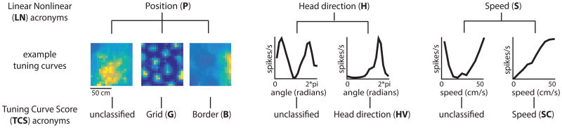
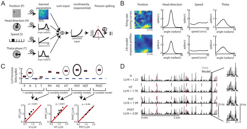
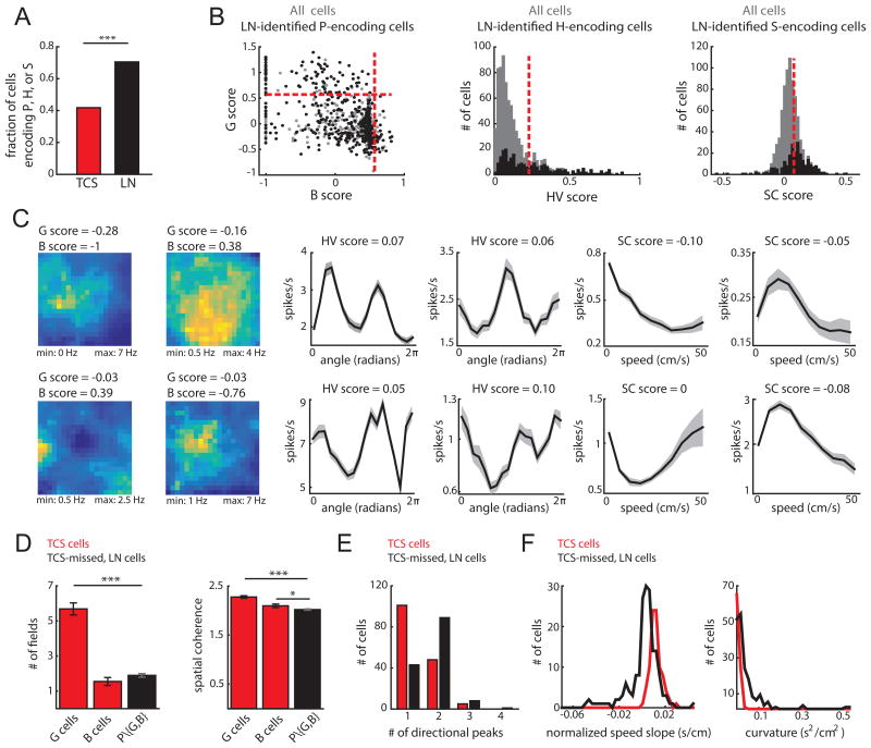
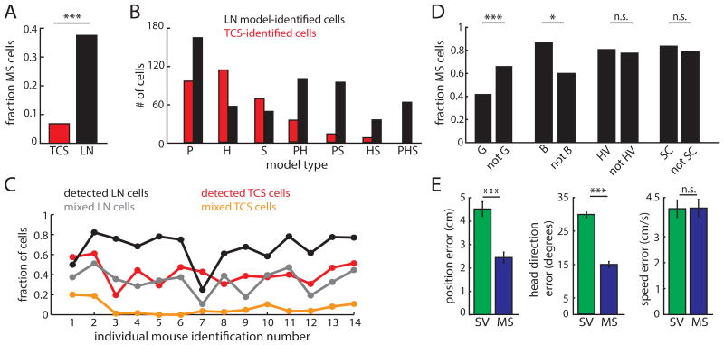
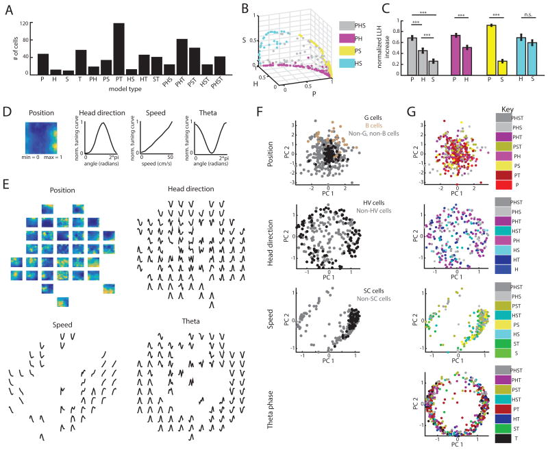
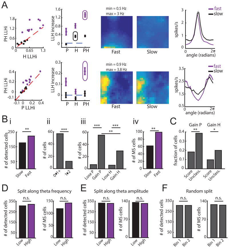
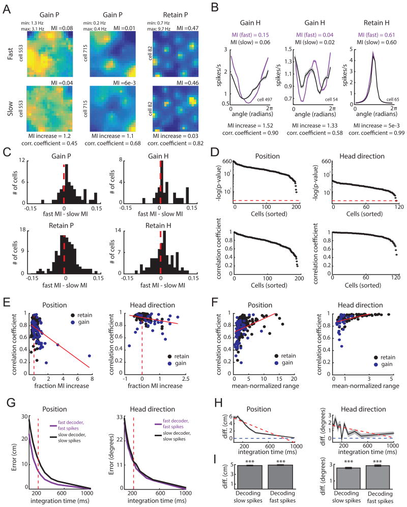
Medial entorhinal grid cells display strikingly symmetric spatial firing patterns. The clarity of these patterns motivated the use of specific activity pattern shapes to classify entorhinal cell types. While this approach successfully revealed cells that encode boundaries, head direction, and running speed, it left a majority of cells unclassified, and its pre-defined nature may have missed unconventional, yet important coding properties. Here, we apply an unbiased statistical approach to search for cells that encode navigationally relevant variables. This approach successfully classifies the majority of entorhinal cells and reveals unsuspected entorhinal coding principles. First, we find a high degree of mixed selectivity and heterogeneity in superficial entorhinal neurons. Second, we discover a dynamic and remarkably adaptive code for space that enables entorhinal cells to rapidly encode navigational information accurately at high running speeds. Combined, these observations advance our current understanding of the mechanistic origins and functional implications of the entorhinal code for navigation. VIDEO ABSTRACT.

Keywords: Multiplexed-coding; adaptive coding; computational models of spatial coding; encoding mode; entorhinal cortex; spatial navigation; tuning heterogeneity.

Figure 1

The LN model approach and the TCS approach represent two distinct ways of characterizing MEC responses. LN method: P = position-encoding cells, H = head direction-encoding cells, S = speed-encoding cells. TCS method: G = grid cells, B = border cells, HV = head direction cells, SC = speed cells. Lines within the chart signify which response profiles are captured by each approach. (See also Figure S1)

Figure 2

The LN model provides an unbiased method for quantifying neural coding. A. Schematic of LN model framework. P, H, S and T are binned into 400, 18, 10, and 18 bins, respectively. The filled bin denotes the current value, which is projected (encircled x) onto a vector of learned parameters. This is then put through an exponential nonlinearity that returns the mean rate of a Poisson process from which spikes are drawn. B. Example firing rate tuning curves (top) and model-derived response profiles (bottom, computed from the PHST model; means from 30 bootstrapped iterations shown in black and the standard deviation in gray). C. Top: Example of model performance across all models for a single neuron (mean ± SEM log- likelihood increase in bits, normalized by the number of spikes [LLHi]). Selected models are circled, with the final selected model in bold. Bottom: comparison of selected models. Each point represents the model performance for a given fold of the cross-validation procedure. The forward-search procedure identifies the simplest model whose performance on held-out data was significantly better than any simpler model (p < 0.05). D. Comparison of the cell's firing rate (gray) with the model predicted firing rate (black) over 4 minutes of test data. Model type and model performance (LLHi) listed on the left. Red lines delineate the 5 segments of test data. Firing rates were smoothed with a Gaussian filter (o = 60 ms). (See also Figures S1 and S2)

Figure 3

The LN model captured coding for the majority of superficial MEC neurons. A. Fraction of cells that encode position, head direction, or running speed based on the TCS (red) or LN (black) approach (*** indicates p < 0.001). B. The tuning-curve scores of cells detected by the LN model (black) as encoding P (left), H (center) and S (right). Score values for all cells are shown in gray. Red lines indicate the TCS 99^th percentile threshold. In total, 307/421 P cells, 141/254 H cells, and 176/242 S cells were not classified as G or B (left), HV (middle) or SC (right) cells, respectively. C. Example model-derived response profiles. P response profiles colored coded for minimum (blue) and maximum (yellow) values (left two columns). H (middle two columns) and S coding (right two columns) are denoted by the mean ± SD of a response profile across 30 bootstrapped iterations of the model-fitting procedure. Models used to compute response profiles: top row: PHS, PS, HS, HST, PHS, ST; bottom row: PST, PST, HST, HS, PST, PST. D. P cells captured only by the LN model (P\{G,B}) had significantly fewer firing fields (left) than G cells (mean field number ± SEM: G = 5.69 ± 0.35, B = 1.55 ± 0.23, P\{G,B} = 1.90 ± 0.10; G and P\{G,B} t-test t(406) = -14.3, p = 5.1e-38; B and P\{G,B} t-test t(347) = 1.2, p = 0.22) and lower spatial coherence (right) than G and B cells (mean coherence ± SEM: G = 2.28 ± 0.03, B = 2.10 ± 0.04, P\{G,B} = 2.02 ± 0.01; G and P\{G,B} t(406) = -9.6, p = 5.7e-20; B and P\{G,B} t-test t(347) = -2.1, p = 0.04). (***p < 0.001; *p < 0.05). E. H cells captured only by the LN model had significantly more peaks in their tuning curves than HV cells (mean peaks ± SEM; HV = 1.37 ± 0.05, H = 1.77 ± 0.05, t-test t(293) = -5.96; p = 7.3e-9). F. S cells captured only by the LN model exhibited negative modulation of firing rate by running speed (left) and significantly higher curvature in their tuning curves than SC cells (mean curvature ± SEM; SC = 0.007 ± 5e-4, S = 0.04 ± 0.005, t-test t(263) = 4.72, p = 3.9e-6). For D-F, *** p<0.001. (See also Figure S3)

Figure 4

Mixed selectivity is a ubiquitous coding scheme utilized by superficial MEC neurons. A. The LN approach (black) reveals significantly more mixed selectivity (MS) for P, H, and S compared to the TCS approach (red). (*** indicates p<0.001.) B. Comparison of model types classified by the LN (black) and TCS (red) methods for navigational variables. C. Proportion of TCS-detected, LN-detected, mixed TCS (cells that cross 2 or more score thresholds), and mixed LN (cells that significantly encode multiple variables) cells for each mouse. D. Comparison of the fraction of model-defined MS cells that either pass, or do not pass, the G, B, HV, or SC thresholds. Number of MS cells/total: G = 36/86, non-G = 221/335; B = 24/28, non-B = 233/393; HV = 90/113, non-HV = 108/141; SC = 55/66, non-SC = 138/176. * indicates p<0.05, *** indicates p<0.001, n.s. = not significant. E. Error in decoding position (left), head direction (middle), and running speed (right) when using either MS or SV cells (n = 332 for both groups; P. *** p < 0.001, n.s. p > 0.5. (See also Figures S3 and S4)

Figure 5

MEC neurons show highly heterogeneous response profile shapes. A. Histogram of the selected models for the 617 cells identified by the LN model approach. B. 3D scatter plot of the normalized contribution of P, H, and S to the model performance of MS cells. Cells are color-coded by model. Variable contributions were measured as the average change in model performance due to addition or deletion of that variable from the selected model (e.g. the contribution of P to a PH neuron is the log-likelihood difference between the H and PH models). C. Mean (± SEM) contribution of P, H, and S for cell-types shown in (B). *** p < 0.001, n.s. = not significant. D. Example of normalized model-derived response profiles. E. For each variable, we constructed a 2-dimensional ‘response-profile’ space, where location in each space is determined by a cell's normalized response profile for that variable. Here, we show the normalized response profiles of a randomly chosen set of cells that were plotted in this space, demonstrating that diverse response profiles vary smoothly across location. Panels F-H use these same four axes to indicate where the response profiles of all the cells lie. F. Projected data, colored according to TCS identification (gray indicates cells not identified by the TCS approach). Each point is a single cell (P: 421 cells, H: 254 cells, S: 242 cells, T: 464 cells). The location of each point is determined by the shape of that cell's response profile. G, HV, and SC cells were significantly clustered for at least one value of k, while B cells trended towards significance for k = 1. G. Same as (F), but colored according the each cell's selected LN model. (See also Figure S5)

Figure 6

Dynamic spatial coding in MEC. A. Example model selection procedures for each epoch. Top row: example cell that encodes H at slow speeds and PH at fast speeds. Bottom row: example cell that gains PH at fast speeds. Both rows; Left: Comparison of model performance for both epochs. Performance (mean ± SEM) of P, H, and PH models during fast and slow epochs with the selected model circled (shown for a single iteration). Middle: Response profiles for P of PH model during fast and slow speeds, color-coded for minimum (blue) and maximum (yellow) values across both epochs. Right: Response profiles (mean ± SD) for H of PH model during fast and slow speeds. B. i. Number of cells encoding P, H, or PH increases at fast speeds. ii. Cells gain coding for P or H at high speeds in two ways. Cells that do not encode P or H at slow speeds encode P, H or PH at fast speeds (0→1+) and cells that encode P or H at slow speeds encode PH at fast speeds (1→2). Significantly more cells fall into the former group (comparison of proportions z = 5.5, p = 3e-8). iii. More cells gain rather than lose P or H at fast speeds; more cells gain P than H. iv. More cells exhibit mixed selectivity at fast speeds. *** p < 0.001, ** p < 0.01, n.s. = not significant. C. Cells unclassified by the TCS method were more likely to gain P or H at fast speeds. ** p < 0.01, * p < 0.05. D.-F. Same as (Bi, ii and iv), but for data split along theta frequency (D), theta amplitude (E) or randomly (F). In the first two cases, speed coverage was matched between epochs. n.s. = not significant. (See also Figures S6 and S7)

Figure 7

Tuning is more informative at fast speeds and is adaptive. A-B. Example response profiles for cells that gain or maintain P or H coding (follows plot conventions of Figure 6). Response profiles, and all comparisons in this figure unless stated otherwise, are derived from the more complex selected model across epochs. For each pair, the mutual information (MI), fractional increase in MI [(MI_fast - MI_slow)/MI_slow], and Pearson correlation coefficients, are computed. C. Difference in MI for position (left) and head direction (right) for cells that gain P (top left) or gain H (top right) at fast speeds, and cells that retain P (bottom left) or retain H (bottom right) across speeds. D. Negative log of p-values (top) and coefficients (bottom) for correlations between the slow and fast-epoch response profiles for cells that gain or retained P or H coding. The red line indicates p = 0.05, with cells above this line attaining significance. E. Scatter plot of MI fractional increase and correlation coefficient between response profiles for cells that gained (blue) or retained (black) P (left) or H (right) coding features with fast speeds. Dashed red line indicates an MI increase of 0, while the solid red line indicates the best-fit line to the data. F. Scatter plot of the mean-normalized range of the slow-derived response profile and correlation coefficients from (E) for cells that gained or retained coding P (left) or H (right) with fast running speeds. G. Top: P and H decoding error of a decoder trained and tested on data derived from parameters of the selected model during fast epochs (purple) versus parameters of the selected model during slow epochs (black). H. Difference in error in decoding position (left) and head direction (right) between the slow and fast decoders in (G). I. Decoding error difference for position (left) or head direction (right) between the slow and fast decoder when decoding data from slow epochs (‘slow spikes’; left of each plot) or when decoding data from fast epochs (‘fast spikes’; right of each plot). Mean difference is computed by averaging across all decoding iterations and tested integration times. Error bars correspond to standard error of the mean across the decoding iterations. *** p < 0.001. (See also Figure S7)

References

1. Atkinson AC, Riani M, Cerioli A. The forward search: Theory and data analysis. Journal of the Korean Statistical Society. 2010;39:117–134.
1. Barak O, Rigotti M, Fusi S. The sparseness of mixed selectivity neurons controls the generalization-discrimination trade-off. Journal of Neuroscience. 2013;33:3844–3856. - PMC - PubMed
1. Bonnevie T, Dunn B, Fyhn M, Hafting T, Derdikman D, Kubie JL, Roudi Y, Moser EI, Moser MB. Grid cells require excitatory drive from the hippocampus. Nat Neurosci. 2013;16:309–317. - PubMed
1. Brun VH, Leutgeb S, Wu HQ, Schwarcz R, Witter MP, Moser EI, Moser MB. Impaired spatial representation in CA1 after lesion of direct input from entorhinal cortex. Neuron. 2008;57:290–302. - PubMed
1. Burak Y, Fiete IR. Accurate path integration in continuous attractor network models of grid cells. PLoS Comput Biol. 2009;5:el000291. - PMC - PubMed