Rapid and coordinated processing of global motion images by local clusters of retinal ganglion cells

Abstract

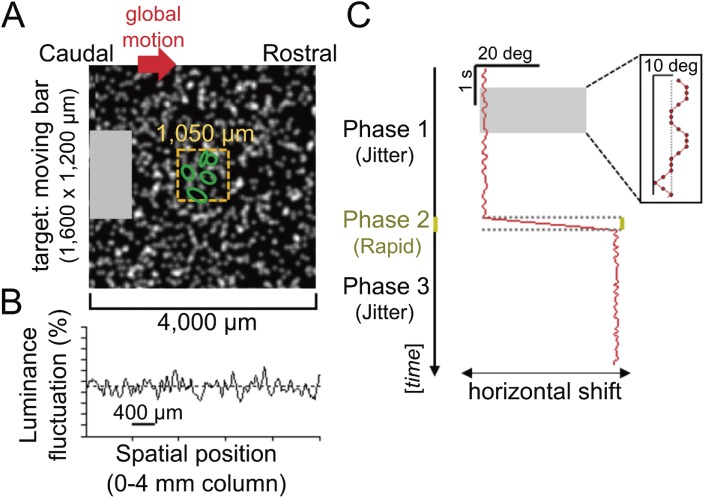
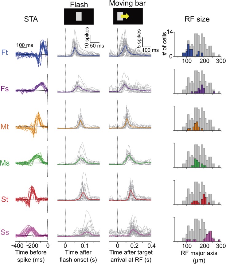
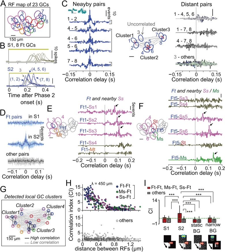
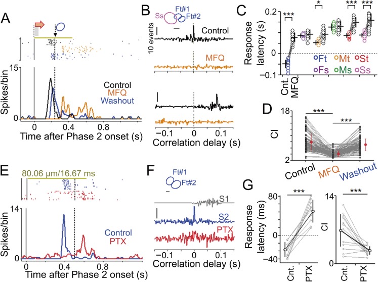
Even when the body is stationary, the whole retinal image is always in motion by fixational eye movements and saccades that move the eye between fixation points. Accumulating evidence indicates that the brain is equipped with specific mechanisms for compensating for the global motion induced by these eye movements. However, it is not yet fully understood how the retina processes global motion images during eye movements. Here we show that global motion images evoke novel coordinated firing in retinal ganglion cells (GCs). We simultaneously recorded the firing of GCs in the goldfish isolated retina using a multi-electrode array, and classified each GC based on the temporal profile of its receptive field (RF). A moving target that accompanied the global motion (simulating a saccade following a period of fixational eye movements) modulated the RF properties and evoked synchronized and correlated firing among local clusters of the specific GCs. Our findings provide a novel concept for retinal information processing during eye movements.

Figure 1.

Global motion images used to simulate eye movements. (A) Motion images (the frame size, 4,000 × 4,000 µm) projected on the ventral retina. The background was uniformly dark (S1) or Gaussian filtered white random-dot array (S2). The target (1,600 × 1,200 µm, 65.6% contrast) moved together with the background horizontally (red arrow). The area of the multi-electrode array (yellow dotted square) and examples of RFs (green ellipses). (B) Spatial luminance fluctuations of the random-dot background. Each value is the mean luminance of 2-column bin. (C) Schema of the S2 sequence. The background was jittered within the frame for ∼4.0 s (Phase 1), then both the target and the background moved rapidly at the same speed (108°/s) toward the center for ∼0.4 s (Phase 2), and finally both stopped and jittered at the center of the frame (Phase 3). The red line shows a trajectory of horizontal motion. Inset, expanded trace in the shaded gray period. Each dot indicates the image position after each refreshment.

Figure 2.

GC classification based on the temporal profile of receptive field. (A) Left, an example of the receptive field (RF) estimated by the spike-triggered average (STA). Right, for eight axes from the RF center pixel (magenta “x” in the left panel), each edge (colored small circles) of the correlated region was defined as the pixel, the intensity of which was higher than the threshold (mean + 6SD of the intensity in uncorrelated regions, dotted black line, see Materials and methods), and then the eight edges were fitted to a 2D ellipse. (B) Temporal profile of the STA. The intensity of STA in each temporal window was computed as the mean of 3 × 3 pixels at the RF center. (C, D) GC classification. Principal component analysis of the temporal STA waves (C). Each STA was projected onto the first and second PCA axes. Eigenvalues of these principal components explain 82.4% of the population variance. Red curves are fitted Gaussians. To interpret these axes, we evaluated several measures of the STA profile (D). For the first PCA axis, the time-to-peak value of the STA profile (D, upper left; top, PCA1st < −0.2; middle, −0.2 < PCA1st < 0.2; bottom, 0.2 < PCA1st) but not the peak value (D, upper right) could explain the main variance of the distribution. For the second PCA axis, the half width of the half maximum of the STA profile could explain the main variance of the distribution (D, lower left; top, PCA2nd < 0; bottom, 0 < PCA2nd). Black triangle, median. Therefore, in the feature space of the STA population, six clusters were discriminated mainly by the time course and duration of the temporal STA profile (C).

Figure 3.

Classification of goldfish GCs based on the temporal profile of receptive field. GCs were classified into 6 groups by the temporal profile of the spike-triggered average (STA, Left): Fast-transient (Ft), Fast-sustained (Fs), Medium-transient (Mt), Medium-sustained (Ms), Slow-transient (St), and Slow-sustained (Ss) GCs. The PSTHs obtained by stationary flash stimulation (1,600 × 1,600 µm, 2 s; Middle left) and by moving bar stimulation (1,600 × 1,200 µm, 6.48 mm/s: 108°/s; Middle right) on a uniformly dark background. The PSTHs from each cell (gray) and the mean (colored). Right, The histograms of RF size (the major axis). Data from all GC groups (gray) and data from each GC group (colored). 119 GCs, 8 retinas.

Figure 4.

Responses to the global motion images evoked by simulated fixational and saccadic eye movements. (A) Stimulus sequence of the S1 (without background, BG) and S2 (the simulated eye movement) conditions. (B) Firing of a Fast-transient (Ft) GC in the S1 (black trace) and S2 (blue trace) conditions. Dotted gray, gray, and yellow lines denote the Phase 1 onset, the Phase 2 onset, and the period of Phase 2, respectively. (C) Expanded (shade in B) traces (lower) and raster plots (upper). Red line, the timing when the target arrived at the edge of RF (ellipse). (D) Raster plots and PSTHs of the Ft GC in the S1 (black) and S2 (blue) conditions. Inset, spike waves (scale bar, 0.2 ms, 100 µV). (E) RF map (upper left) and PSTHs obtained from 15 simultaneously recorded GCs (lower left and right) in the S1 (gray) and S2 (colored) conditions. Each color designates the corresponding GC group in this and the following Figures. (F) A plot of the response latency in the S2 condition against that in the S1 condition (81 GCs, 5 retinas). The negative value indicates that the response is evoked before the target arrives at the RF edge. (G) Peak firing rate in Phase 2. Black and gray thick bar, mean ± SE. 102 GCs, 6 retinas. *, p < 0.05. ***, p < 0.001. Paired t-test with Bonferroni correction.

Figure 5.

Effects of background on the response latency to the rapidly moving target in the S2 condition. (A) A plot of the response latency to the moving target in the condition where the background (BG) during Phase 1 was immobilized (static BG, ordinate) against that in the S1 condition (abscissa). (B) Effects of the background size on the response latency of Ft GCs (49 cells, 5 retinas). Negative response latency was observed when the size was larger than 3.2 × 3.2 mm (p < .05, Binormal test). Red circle and red bar, mean ± SD. (C) The response latency to the rapidly moving target (Phase 2 in the S2 condition) was affected by background contrast of the random-dot pattern. Ft GCs responded with negative latency when the background contrast was in the range between 5 and 60%. 25 Ft GCs. (D) In any background contrast condition, negative response latency was not observed in other GCs (5 Fs, 8 Mt, 12 Ms, 16 St, and 38 Ss GCs). Note that in the high background contrast condition (70 and 80%, i.e., high background intensity) the moving target did not evoke spikes (filled circles), suggesting the response saturation. Data from 3 retinas.

Figure 6.

Spatial spread of the response modulation. (A) RF map and the stop position of global rapid motion (Phase 2). In the Stop@1 condition (dotted gray line), the target covered all RFs. In the Stop@2 condition (dotted yellow line), the target partially covered only the RF of Ss#1 and St#2. (B) Responses in the S1 (upper) and S2 (lower) conditions. The PSTHs were obtained in the Stop@1 (light gray) and Stop@2 (colored) conditions. Ft#4 responded in the S2 condition even when the target stopped well short of its RF (red arrow). Horizontal lines, the period of target motion (black, the Stop@1; yellow, the Stop@2). Gray vertical line, the Phase 2 onset. Red dotted line, timing of the target arrival at each RF. Yellow dotted line, timing of the stop of global motion in the Stop@2 condition. (C) Response index as a function of distance between the leading edge of the target and the RF edge in the S1 (upper) and S2 (lower) conditions (49 GCs, 4 retinas).

Figure 7.

Coordinated firing in a local cluster of GCs during global rapid motion. (A) RF map on a ventral retina. (B) The PSTHs in Phase 2 obtained from 8 Ft GCs in the S1 (upper) and S2 (lower) conditions. (C) The cross-correlograms (the noise correlation) in Phase 2 calculated from the nearby (left) and distant (right) Ft GC pairs. RF map and schematic correlation between Ft GCs in the S2 condition (middle). Pairs with high (red) and low (dotted gray) correlation. (D) The noise correlation in 8 Ft GC pairs (blue, mean; light blue, SD) in the S1 (top), S2 (middle) conditions, and that in pairs of other GCs in the S2 condition (bottom). (E, F) RF map (left) and the noise correlation (right) calculated from pairs of the Ft GC and a GC of other GC groups (reference neuron: E, Ft#1; F, Ft#5). The peak appeared at a positive correlation delay (arrow). (G) Local GC clusters with high noise correlation. (H) Relation between the center-to-center RF distance and the correlation index (CI) in the S2 condition (127 GCs, 729 pairs, 8 retinas). λ, the distance constant. (I) CIs in the S1, S2, the static background (BG), and the narrow BG conditions. Mean ± SD. Dotted green line, the mean CI of the raw cross-correlograms calculated from the firing to stationary flash illumination.

Figure 8.

Stimuli having the characteristics of in vivo eye movements induce the response modulation. (A) After Phase 1 (left), both the target and the background were rapidly moved in one of four cardinal directions (right) in the S1 (upper) and S2 (lower) conditions. (B) The PSTHs of a Ft GC in the S1 (upper) and S2 (lower) conditions. Gray dotted line, timing of the target arrival at the RF edge. (C) Direction selectivity in the S1 (black) and S2 (blue) conditions. The mean firing rate (upper) and the mean response latency (lower) to the target. 19 Ft GCs, 4 retinas. Filled circle and error bar, mean ± SD. (D) The noise correlation in the S2 condition (blue, Ft#2-Ft#3 pair; magenta, Ss#1-Ft#3 pair). Horizontal motion (upper) and vertical motion (lower). RF map (top). Scale bar, 100 µm. (E) Effects of motion direction on the correlation index (CI) in the S2 condition. Error bar denotes SD. (F) Effects of motion velocity on the response latency to the target. 9 Ft GCs, 3 retinas. Small circle, the response latency of each Ft GC. Colored circle and error bar, mean ± SD. Velocity range of in vivo saccades (shaded area, see 27, 28). (G) Effects of duration of global jitter motion in Phase 1 on the response latency to the target in Phase 2. Red, mean ± SD. 28 Ft GCs, 6 retinas. Green shaded area, the range of jitter duration in in vivo fixational eye movements (cyan dotted line, the median duration 2.03 s, see 28). Data plotted on an expanded time scale (right). (H) RF map (top) and the noise correlation in Phase 2 (middle and bottom). Global jitter motion in Phase 1 lasted for 2 s (gray) or 0.75 s (colored). Scale bar, 100 µm. (I) Relation between the duration of global jitter motion and the CI. 48 GCs, 195 pairs, 3 retinas.

Figure 9.

Effects of a gap junction blocker and a GABA antagonist on the response modulation. (A) Effects of a gap junction blocker, mefloquine (MFQ, 10 µM). Firing of a Ft GC before (black, control), during (orange, MFQ), and after (blue, Washout) application of MFQ. Gray, yellow, and dotted gray lines indicate the Phase 2 onset, the period of Phase 2, and the timing of the target arrival at the RF edge, respectively. (B) The noise correlation calculated from Ft#2-Ft#1(upper) and Ss-Ft#1 (lower) pairs in the control (black) and MFQ (yellow) conditions. (C) Response latency in the control (colored) and MFQ (black) conditions (76 GCs, 4 retinas). Black and gray bar, mean ± SD. (D) Effects of MFQ on the CIs calculated from Ft-Ft, Ms-Ft, and Ss-Ft GC pairs (124 pairs). Red, mean ± SD. (E, F) Effects of a GABA antagonist, picrotoxin, (PTX, 100 µM). Blue, control. Red, PTX. Firing in Phase 2 (E) and the noise correlation of the Ft GC pair (F). (G) Effects of PTX on the response latency (left, 10 Ft GCs, 3 retinas) and the correlation index (CI) (right, 13 Ft pairs, 3 retinas). *, p < 0.05. ***, p < 0.001. Paired t-test with Bonferroni correction.

References

1. Land M. (1992) Predictable eye-head coordination during driving. Nature 359, 318–320. - PubMed
1. Martinez-Conde S., Macknik S., Hubel D. (2004) The role of fixational eye movements in visual perception. Nat. Rev. Neurosci. 5, 229–240. - PubMed
1. Wurtz R. (2008) Neuronal mechanisms of visual stability. Vision Res. 48, 2070–2089. - PMC - PubMed
1. Lee D., Malpeli J. (1998) Effects of saccades on the activity of neurons in the cat lateral geniculate nucleus. J. Neurophysiol. 79, 922–936. - PubMed
1. Reppas J., Usrey W., Reid R. (2002) Saccadic eye movements modulate visual responses in the lateral geniculate nucleus. Neuron 35, 961–974. - PubMed