Mechanics of ultrasound elastography

Abstract

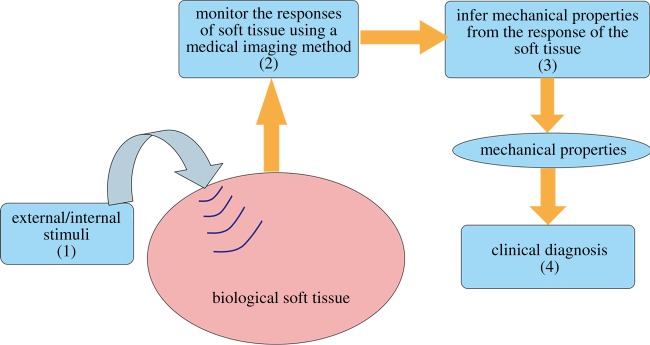
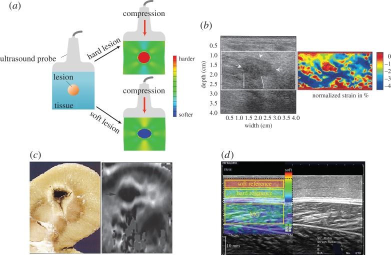
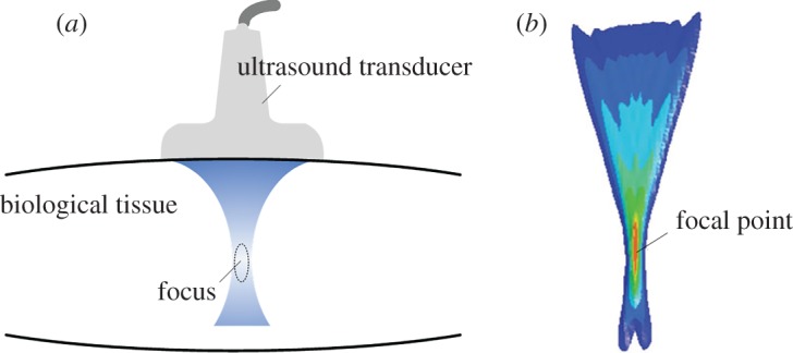
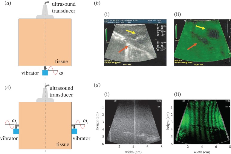
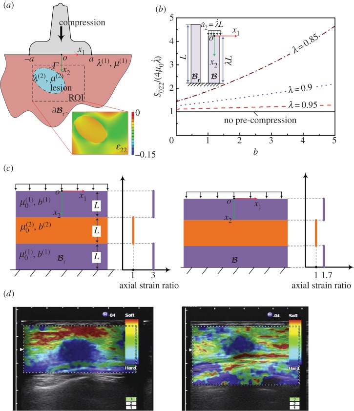
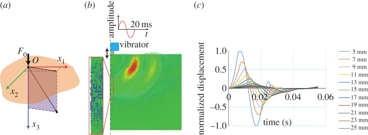
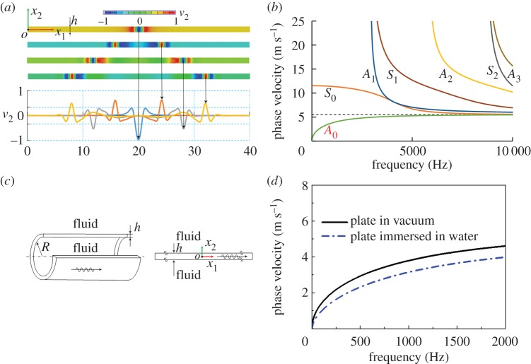
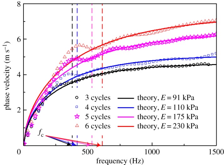
Ultrasound elastography enables in vivo measurement of the mechanical properties of living soft tissues in a non-destructive and non-invasive manner and has attracted considerable interest for clinical use in recent years. Continuum mechanics plays an essential role in understanding and improving ultrasound-based elastography methods and is the main focus of this review. In particular, the mechanics theories involved in both static and dynamic elastography methods are surveyed. They may help understand the challenges in and opportunities for the practical applications of various ultrasound elastography methods to characterize the linear elastic, viscoelastic, anisotropic elastic and hyperelastic properties of both bulk and thin-walled soft materials, especially the in vivo characterization of biological soft tissues.

Keywords: shear wave; soft tissues; ultrasound elastography.

Figure 1.

An illustration of the key steps involved in elastography [8]. (Online version in colour.)

Figure 2.

(a) Illustration of the basic principle underlying static elastography. (b) Detection of a breast lesion, which appears as the low-strain region in the image. Compared with the B-mode image, the elastography method may provide more accurate information with respect to both the size and the position of a lesion [45]. (c) Application of static elastography to image a thermal lesion induced by HIFU, revealing that this technique may be useful to guide HIFU treatment [46]. (d) Measurement of the elastic properties of skeletal muscles using the static elastography method. To quantitatively infer the elastic properties of the muscle, two soft layers with known mechanical properties are used [47]. Reprinted from references [45], [46], and [47] with permission. (Online version in colour.)

Figure 3.

(a) Schematic of the ARF in biological soft tissues induced by a focused ultrasound beam. (b) The isocontours of the ARF distribution from a focused linear array in a soft medium; here the acoustic attenuation coefficient is 0.7 dB cm⁻¹ MHz [52]. Reprinted from reference [52] with permission. (Online version in colour.)

Figure 4.

(a) Schematic of sonoelastography. (b) The B-mode image (i) and vibration amplitude map (ii) obtained via sonoelastography of a porcine liver with a thermal lesion [5]. (c) Schematic of crawling wave imaging. (d) The B-mode image (i) and a frame showing the crawling waves (ii) in a phantom consisting of a hard layer (left) and soft layer (right) [81]. Reprinted from references [5] and [81] with permission. (Online version in colour.)

Figure 5.

(a) Schematic of the SWIRE. (b) Typical frequency-domain displacement curves at a point within the soft inclusion, from which the resonance frequency can be determined from the peaks in the curves. The stationary shear wave displacement field in the ROI at the resonance frequency is also presented [61]. Reprinted from reference [61] with permission. (Online version in colour.)

Figure 6.

(a) Schematic of VA. (b) The amplitude and phase acoustic spectrograms of normal and calcified excised human iliac arteries obtained using the VA method [62]. (c) Schematic of HMI. (d) The HMI displacement variation and corresponding pathology images of liver tissue for 30 s of sonication [71]. Reprinted from references [62] and [71] with permission. (Online version in colour.)

Figure 7.

(a) Schematic SDUV [74]. (b) Dispersion curve of a phantom. The points were obtained from experiments, and the solid line is the least mean square fitting result. The viscoelastic parameters of the phantom determined using the SDUV method agree well with those obtained from an independent measurement [74]. Reprinted from reference [74] with permission.

Figure 8.

(a) Schematic of TE [17]. (b) Propagation of the transient elastic waves in livers with different degrees of fibrosis. The results from left to right are for F₀, F₂ and F₄. The velocities of the transient waves can be deduced from the slope of the white dotted lines: a steeper line indicates a faster wave [17]. Reprinted from reference [17] with permission. (Online version in colour.)

Figure 9.

(a) Schematic of the SWEI method [18]. (b) The shear waves recorded by the MRI [18]. (c) The shear waves recorded via the AFRI-based SWEI method, showing the displacements along the lateral direction at different times. Clearly, the displacements are attenuated along the propagation direction [94]. (d) Normalized displacement map obtained from (c); based on the slope of the bright line, the shear wave velocities can be evaluated [94]. Reprinted from references [18] and [94] with permission.

Figure 10.

(a) The displacement field given by FEA, indicating the formation of the shear-wave Mach cone. In this case, the moving velocity of the vibration source is three times the velocity of the shear wave in the target material. (b) The propagation process of the interfered wavefronts within 14 ms after applying the ARF recorded during an experiment on a phantom [20]. (c) The in vivo elastogram obtained via SSI for breast tissues [95]. (d) A photograph of the Aixplorer® ultrasound instrument (Supersonic Imagine, Aix-en-Provence, France). Reprinted from references [20] and [95] with permission. (Online version in colour.)

Figure 11.

(a) ARFs generated by multi unfocused ultrasound beams. (b) Shear waves generated by CUSE in a homogeneous phantom. Panels (c) and (d) give the shear wave velocity maps in the whole FOV for a homogeneous phantom and a phantom with a hard inclusion, respectively [96]. Reprinted from reference [96] with permission. (Online version in colour.)

Figure 12.

(a–c) The axial components of the partical velocities in a vessel-mimicking phantom overlaid on the B-mode image at approximately 0.2, 0.8 and 1.4 ms after the action of the ARF. The inner radius and wall thickness of the vessel-mimicking phantom are 2 mm and 1 mm, respectively. (d) The solid line along which the spatio-temporal imaging of the shear wave propagation occurred is shown in (e). (f) The dispersion curve derived from spatio-temporal imaging via a two-dimensional Fourier transformation [119]. (Online version in colour.)

Figure 13.

(a) Schematic of the mechanical model underlying static elastography and the axial strain in the ROI calculated by FEA (${\dot{u}}_2=0.1a$). The inclusion in the ROI is harder than the surrounding tissue. (b) Effect of pre-compression on the elastic modulus measured via static elastography. (c) Illustration of the decrease in the axial strain image contrast caused by pre-compression. The ratio of the initial shear moduli of the two materials is μ⁽²⁾/μ⁽¹⁾ = 3. A 10% pre-compression will cause the strain ratio to decrease from 3 to 1.7. (d) The decrease of the strain image contrast due to the excessive compression observed in the experiment of Shiina et al. [39]. Reprinted from reference [39] with permission. (Online version in colour.)

Figure 14.

(a) Schematic of the Lamb problem (i.e. the motion of a half-space induced by a concentrated force). (b) Typical displacement field in the TE given by FEA. The frequency of the vibrator is 50 Hz and the loading process lasts 20 ms. (c) The axial displacements of the points on the axis at different depths (5 ∼ 25 mm). The displacements are normalized by the displacement at the depth of 5 mm. Based on the arrival times of the displacement peaks, the velocity of the transient wave can be determined. (Online version in colour.)

Figure 15.

(a) Propagation of guided waves in an elastic plate. When the transient shear waves generated at the centre of the plate propagate in opposite directions, the wavefronts change constantly. (b) Dispersion relation of the antisymmetric and symmetric modes of the Lamb wave. (c) The simplified model used in GWE of the arterial wall. (d) The dispersion relations of the A₀ mode in elastic plates in vacuum and immersed in water. (Online version in colour.)

Figure 16.

Experimental results (discrete points) obtained from vessel-mimicking phantoms with different elastic moduli are fitted with equation (3.55) (solid lines). The vessel-mimicking phantoms were made from polyvinyl alcohol cryogel which underwent different freezing/thawing cycles, i.e. three to six cycles, and had different elastic moduli. Both the critical frequencies and the elastic moduli of the phantoms are determined according to the method suggested in [119]. (Online version in colour.)

Figure 17.

Plot of the phase velocity. Because v_qSV is axisymmetric, only the distribution of v_qSV in the x₁–x₃-plane is plotted. For all three cases, μ_T = 9 kPa, μ_L = 25 kPa, and the parameter C is (a) 62.5 kPa, (b) 0 and (c) −21.875 kPa, respectively. (Online version in colour.)

Figure 18.

FE simulation of shear wave propagation in TI materials with different values of C. For all three cases, μ_T = 9 kPa, and μ_L = 25 kPa. The direction of the focused ARF is applied along the Z-axis, which has a 45° angle with the x₃-axis (fibre direction) [35]. Reprinted from reference [35] with permission. (Online version in colour.)

Figure 19.

The ECE at a high Mach number when the angle between the direction of the moving force (Z-axis) and the fibre direction (x₃-axis) is taken as 45°. (a,d,g) C > 0; (b,e,h) C = 0; (c,f,i) C < 0. For all three cases μ_T = 9 kPa, and μ_L = 25 kPa [34]. (Online version in colour.)

Figure 20.

The SSI-based experimental protocol used to fully characterize skeletal muscles. (a,d) The SH mode shear wave is generated along the fibre direction and its velocity, $c_{\mathrm{SH},\parallel }$, is measured. According to equation (3.59), μ_L can be measured as ${\mu }_{\mathrm{L}}=\rho c_{\mathrm{SH},\parallel }^2$. (b,e) Similarly, μ_T can be measured using the SH mode shear wave propagating perpendicular to the fibre according to ${\mu }_{\mathrm{T}}=\rho c_{\mathrm{SH},\mathrm{\perp }}^2$. (c,f) In this step, the velocity of the qSV mode shear wave, $c_{{\mathrm{qSV},45}^{\circ }}^{}$, is measured. Then E_L can be determined as $E_{\mathrm{L}}=4\rho c_{{\mathrm{qSV},45}^{\circ }}^2-{\mu }_{\mathrm{T}}$ [33]. (Online version in colour.)

Figure 21.

Schematic of the finite deformation of the tested material and the wave propagation. (Online version in colour.)

Figure 22.

(a) Dependence of the wave speed on parameter ξ for different λ. (b) The velocities of the shear waves in breast tissues before and after compression. (c) Variation of the shear wave velocities with compression strains determined by SSI, which can be fitted with equation (3.66) to obtain b [8]. (Online version in colour.)

Figure 23.

Experimental results obtained for three patients: a healthy volunteer, a patient with a tumour and a patient with a benign lesion. (a,d,g) B-mode images, (b,e,h) shear moduli and (c,f,i) nonlinear parameter A values [28]. Reprinted from reference [28] with permission. (Online version in colour.)

Figure 24.

The shear wave velocities of the beef ex vivo (a) before and (b) after compression. (c) By fitting the variation of the shear wave velocities with the compression strain, the parameter c₂ was determined [33]. (Online version in colour.)

Figure 25.

Axial-shear strain images from FEM of (a) a firmly bonded inclusion and (b) a loosely bonded inclusion. The coefficient of friction was 0.01, and the applied axial strain was 2%. The inclusion was twice stiffer than the background in both cases [186]. Reprinted from reference [186] with permission. (Online version in colour.)

References

1. Gao L, Parker KJ, Lerner RM, Levinson SF. 1996. Imaging of the elastic properties of tissue—a review. Ultrasound Med. Biol. 22, 959–977. (doi:10.1016/S0301-5629(96)00120-2) - DOI - PubMed
1. Ophir J, Alam SK, Garra B, Kallel F, Konofagou E, Krouskop T, Varghese T. 1999. Elastography: ultrasonic estimation and imaging of the elastic properties of tissues. Proc. Inst. Mech. Eng. H 213, 203–233. (doi:10.1243/0954411991534933) - DOI - PubMed
1. Greenleaf JF, Fatemi M, Insana M. 2003. Selected methods for imaging elastic properties of biological tissues. Annu. Rev. Biomed. Eng. 5, 57–78. (doi:10.1146/annurev.bioeng.5.040202.121623) - DOI - PubMed
1. Sarvazyan A, Hall TJ, Urban MW, Fatemi M, Aglyamov SR, Garra BS. 2011. An overview of elastography – an emerging branch of medical imaging. Curr. Med. Imaging Rev. 7, 255–282. (doi:10.2174/157340511798038684) - DOI - PMC - PubMed
1. Parker KJ, Doyley MM, Rubens DJ. 2011. Imaging the elastic properties of tissue: the 20 year perspective. Phys. Med. Biol. 56, R1 (doi:10.1088/0031-9155/56/1/R01) - DOI - PubMed