An algorithm for separation of mixed sparse and Gaussian sources

Abstract

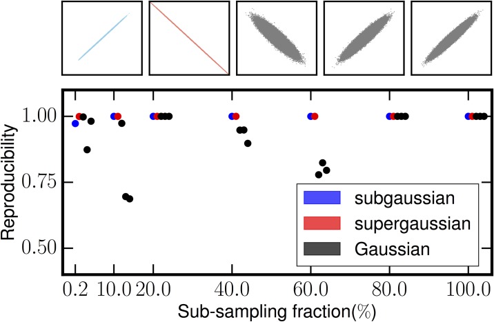
Independent component analysis (ICA) is a ubiquitous method for decomposing complex signal mixtures into a small set of statistically independent source signals. However, in cases in which the signal mixture consists of both nongaussian and Gaussian sources, the Gaussian sources will not be recoverable by ICA and will pollute estimates of the nongaussian sources. Therefore, it is desirable to have methods for mixed ICA/PCA which can separate mixtures of Gaussian and nongaussian sources. For mixtures of purely Gaussian sources, principal component analysis (PCA) can provide a basis for the Gaussian subspace. We introduce a new method for mixed ICA/PCA which we call Mixed ICA/PCA via Reproducibility Stability (MIPReSt). Our method uses a repeated estimations technique to rank sources by reproducibility, combined with decomposition of multiple subsamplings of the original data matrix. These multiple decompositions allow us to assess component stability as the size of the data matrix changes, which can be used to determinine the dimension of the nongaussian subspace in a mixture. We demonstrate the utility of MIPReSt for signal mixtures consisting of simulated sources and real-word (speech) sources, as well as mixture of unknown composition.

Fig 1. Schematic for MIPReSt.

MIPReSt runs the RAICAR algorithm on both the original data matrix X and many random subsamples of smaller column dimension. Comparison of the reproducibilities from the original data and the random subsamples determines the size of the sparse subspace. After projecting that subspace out of X, singular value decomposition $\tilde{X}$, along with an eigenvalue selection rule, produces both the dimension of the Gaussian subspace and a basis for that subspace. (See Methods for details.).

Fig 2. Examples of super- and subgaussian sources.

Shown here are histograms for a Gaussian source (black), a subgaussian source (the generalized Gaussian), and a supergaussian source (Laplace). Also shown is a histogram for one of the speech signals used in this study. The speech signal is far more leptokurtic than the Laplace source; without truncating the y-axis the massive spike near zero of the speech signal obscures the shapes of the other distributions.

Fig 3. Full rank extraction.

We constructed a simulated data matrix with five sources: one supergaussian, one subgaussian, and three Gaussian sources. The simulated data matrix had 5 × 10⁵ samples. The main panel shows the results of RAICAR extractions at different levels of decimation, including the parent data. The best assignment match to the supergaussian source is shown in blue and to the subgaussian source in red. While the Gaussian sources may sometimes have extrememly high reproducibility, they show poor stability when the data is decimated, in constrast to the sparse sources. The top panel shows scatter plots of the estimated sources from the parent data against their best assignment match; the sparse sources are recovered perfectly by RAICAR.

Fig 4. Reproducibility (R) and reproducibility fluctuations (δ_ij) from overextraction.

Only five sources (Gaussian or otherwise) are present, but the mixture dimension is ten. Horizontal bars are located at the median value. There are clearly three groups of sources here. Two sources (the recovered sparse sources) have near-perfect R that does not fluctuate from decimation-to-decimation. Three sources have occasionally high reproducibility, but also significant δ_ij; these are the Gaussian subspace. The remaining five sources have very low reproducibility that fluctuates very little; these sources are spurious sources resulting from overextraction.

Fig 5. Reproducibility (R) and reproducibility fluctuations (δ_ij) for speech signals mixed with Gaussian sources.

For each of the fifteen extracted sources, R is shown in red and δ_ij in black. For both quantities, values for each of the fifty subsampled data matrices are shown as points and the median value as a horizontal bar. The sources clearly group into three categories: high R with low δ_ij (true sparse sources), variable R with high δ_ij (Gaussian sources), and low R and δ_ij (spurious sources).

Fig 6. Reproducibility plot for the Iris data.

The format and color scheme for this figure is identical to that used in Figs 4 and 5. Based on this information and related discussion in the text, it appears that there is one (and likely only one) sparse source present in the iris data.

Fig 7. Histograms of extracted sources from the Iris data.

Each panel shows a histogram (bars) and kernel density estimate (Gaussian kernel, solid line) for one of the four RAICAR sources extracted from the iris data. The nongaussianity of the most reproducible source (upper left) is clearly evident.