Iterative expansion microscopy

Abstract

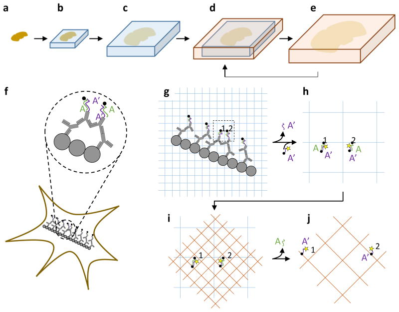
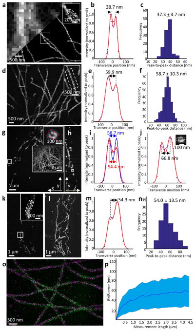
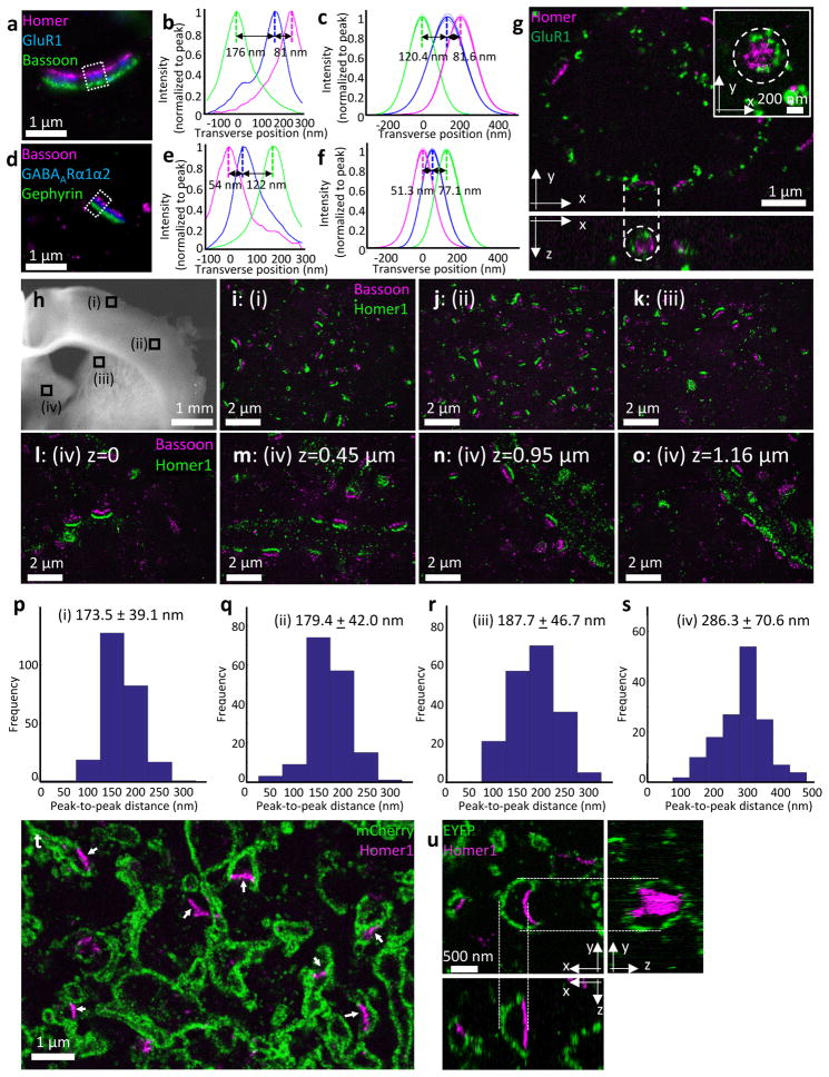
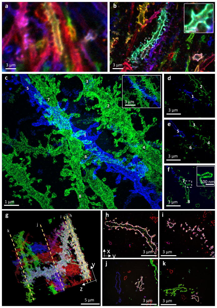
We recently developed a method called expansion microscopy, in which preserved biological specimens are physically magnified by embedding them in a densely crosslinked polyelectrolyte gel, anchoring key labels or biomolecules to the gel, mechanically homogenizing the specimen, and then swelling the gel-specimen composite by ∼4.5× in linear dimension. Here we describe iterative expansion microscopy (iExM), in which a sample is expanded ∼20×. After preliminary expansion a second swellable polymer mesh is formed in the space newly opened up by the first expansion, and the sample is expanded again. iExM expands biological specimens ∼4.5 × 4.5, or ∼20×, and enables ∼25-nm-resolution imaging of cells and tissues on conventional microscopes. We used iExM to visualize synaptic proteins, as well as the detailed architecture of dendritic spines, in mouse brain circuitry.

Figure 1. Iterative expansion microscopy (iExM) concept

(a–e) Schematic of iterative expansion, showing how a brain slice can be expanded multiple times. First, a swellable polyelectrolyte gel network containing a cleavable crosslinker is formed throughout a brain slice (b), then mechanically homogenized and expanded (c), as in our original ExM protocol. After expansion, a second swellable polyelectrolyte gel network is formed throughout the first (d), and then expanded after dissolving the first gel (e). This process (d,e) can be applied repeatedly to increase the physical magnification still further, if desired. (f–j), Molecular view of the iExM process. (f) Biomolecules of interest (gray circles) are first labeled with a primary antibody (shown also in gray) followed by a DNA (purple, sequence A′)-conjugated secondary antibody, then a complementary DNA (green, sequence A) bearing a gel-anchoring moiety (acrydite; black dot), as in our original ExM procedure. (g) The sample is then embedded in a swellable polyelectrolyte gel (blue mesh), which critically involves a chemically cleavable crosslinker. This gel incorporates the DNA of sequence A at the gel-anchoring site, and is expanded. The sample is re-embedded in a charge-neutral backbone polymer (not shown, for simplicity) with a cleavable crosslinker to enable new electrolyte monomers to be infused, and to support DNA hybridization without shrinkage. (h) In order to enable a second round of expansion, a DNA oligo with the original A′ sequence (purple strand), but now bearing a fluorophore (yellow star) and a new gel-anchoring moiety (acrydite; black dot), is hybridized to the anchored A-sequence DNA (green). (i) A second swellable gel (orange mesh) is formed, this time with an uncleavable crosslinker. This gel incorporates the final fluorophore-bearing DNA oligo (sequence A′, purple). (j) The gel expands the labels away from each other after digesting the first and re-embedding gel through crosslinker cleavage.

Figure 2. Validation of the nanoscale precision of iterative expansion microscopy

(a-c) STORM imaging of cultured BS-C-1 cells after microtubules were labeled with an anti-tubulin antibody. (a) Epifluorescence image (upper left) and STORM image (lower right) of microtubules before expansion. The inset in upper right zooms in on the small box at center. (b) Transverse profile of microtubules in the boxed region (dotted lines) of the inset of a after averaging down the long axis of the box and then normalizing to the peak value (blue dots), with superimposed fit with a sum of two Gaussians (red lines). (c) Population data for 110 microtubule segments from two samples (mean ± standard deviation), showing a histogram of peak-to-peak distances. (d–j) Confocal imaging of cultured BS-C-1 cells with labeled microtubules, after ~20-fold expansion via iExM. (d) Single xy-plane image at the bottom of the cell. The inset in upper right zooms in on the small box at left. (e) As in b, but for the inset of d. (f) As in c, but for iExM-processed BS-C-1 cells. n=307 microtubule segments from one expanded sample. (g) Single xy-plane image 1.6 μm above the bottom of the cell. The inset in upper right zooms in on the small box indicated at left, highlighting the circular cross-section of the microtubule (blue and red boxes are used to calculate the profile of i). The large inset at right shows the entire cellular context, as a maximum intensity projection of the sample. (h) Single yz-plane within the volume imaged in g; the small box is highlighted in the inset of j. (i) Transverse profiles (i.e., plotting along the long axis of the highlighting box) of the microtubule in the upper right inset of g, with color corresponding to that of the highlighting box in the inset. (j) Transverse profile of the microtubule in the small box of h. Inset, zoomed-in image of the box of h, showing the cross-section of the microtubule being resolved along the optical axis. (k) Confocal image of a 100-μm thick slice of mouse cortex with microtubules labeled, after ~18-fold expansion via iExM, and imaged at a single xy-plane. (l) Maximum-intensity projection of the sample shown in k. (m) As in e, but for the inset of k. (n) Population data for 96 microtubule segments from one expanded sample, showing a histogram of the peak-to-peak distances. (o) Overlay, using only a rigid registration, of a STORM image (magenta) of cultured BS-C-1 cells stained with anti-tubulin pre-expansion, with a confocal image (green) of the same sample post-expansion. (p) RMS length measurement error of biological measurements, calculated using the distortion vector field method, using STORM microscopy pre-expansion followed by confocal imaging of iExM-processed samples (~20x expanded) (blue line, mean; shaded area, ± 1 standard deviation; n = 3 samples).

Figure 3. Nanoscale resolution imaging of synapses using iExM

(a) Epifluorescence image of cultured hippocampal neurons stained with antibodies against Homer1 (magenta), Glutamate receptor 1 (GluR1, blue), and Bassoon (green), after ~13-fold expansion via iExM and DNA hybridization-based signal amplification. Boxed regions are analyzed further in b. (b) Transverse profile of the three proteins imaged in the sample of a (in the boxed region), after normalizing to the peak (Homer1 in magenta, GluR1 in blue, Bassoon in green). (c) Sum of Gaussian functions fitted to curves as in b, for 10 synapses from one sample, normalized to peak (thick lines, mean; thin lines, ± 1 standard deviation). (d) As in a, but stained with antibodies against Bassoon (magenta), GABA_ARα1/α2 (blue), and Gephyrin (green) (e) As in b, but for the boxed region in d (Bassoon in magenta, GABA_ARα1/α2 in blue, Gephyrin in green). (f) As in c, but for the labels of d; 14 synapses from one sample. (g) Confocal z-stack (top, a single xy-plane; bottom, a single xz-plane; dotted lines connect corresponding points in the two cross-sections) of cultured hippocampal neurons with labeled Homer1 (magenta) and Glutamate receptor 1 (GluR1, green), after ~20-fold expansion via iExM. Inset of upper panel shows a zoomed-in image of a synapse (from another field of view) showing the circular distribution of GluR1 around Homer1. (h) low magnification widefield image of a mouse brain slice (corresponding to slide 57 of the Allen Brain Reference Atlas, P56 mouse, coronal sections) showing four regions i–iv that were imaged after expansion in i–o: (i,ii) primary somatosensory cortex, (iii) dorsal striatum, (iv) medial pallidum. (i–k) Confocal images of three regions (i), (ii), (iii) highlighted in h after labeling with anti-Bassoon (magenta) and anti-Homer1 (green), and 16-fold expansion via iExM. (l–o) Single xy-plane imaged at iv in h, at different z-heights. (p–s) Population data of the Homer1-Bassoon separation (mean ± standard deviation) measured in the four regions shown in h. The number of Homer1-Bassoon pairs analyzed was p, 248 pairs from one specimen; q, 159 pairs from one specimen; r, 189 pairs from one specimen; s, 147 pairs from one specimen. (t,u) Confocal images of motor cortex areas (t, slide 57 of the Allen Brain Reference Atlas P56 mouse coronal sections; u, slide 47 of the same Atlas) after immunostaining and expansion. (t) Confocal image of the specimen after immunostaining with antibodies against Homer1 (magenta) and mCherry (green) and 16-fold expansion via iExM. (u) Z-stack confocal image of the specimen after immunostaining with antibodies against Homer1 (magenta) and EYFP (green) and 20-fold expansion via iExM. Upper left shows a single xy-plane image; right shows a single yz-plane image reconstructed from the z-stack image; bottom shows a single xz-plane image reconstructed from the z-stack image.

Figure 4. Nanoscale imaging of mouse hippocampal brain circuitry

(a) Confocal image of immunostained Emx1-Cre mouse hippocampus with neurons expressing membrane-bound fluorescent proteins (Brainbow AAVs) before expansion. Blue: EYFP, Red: TagBFP, and Green: mTFP. (b) As in a, but expanded 4.5-fold by the antibody anchoring form of the ProExM protocol. Blue: EYFP, Red: TagBFP, Green: mTFP. Inset shows a magnified image of a spine in the dotted box of b. (c–f) Confocal z-stack image of 20-fold expanded mouse hippocampal circuitry with labeled EYFP (blue) and mCherry (green). (c) Maximum intensity projection of the stack shown in (d–f); numbers refer to neural processes that are highlighted within individual z-stacks in (d–f). Inset shows a de–magnified view of the image of (c), with the same scale bar with a and b. (d–f) Single xy-plane images at different z-heights from the bottom of the specimen. (d) z=1.9 μm; (e) z=2.4 μm; (f) z=3.2 μm. See Supplementary Video 5 for 3-D video and surface rendering. Inset of f shows a magnified view of a spine in the dotted box of f. (g–k) Confocal z-stack image of 20-fold expanded mouse hippocampal circuitry with labeled EYFP and mTFP (blue; both EYFP and mTFP were labeled in a same color), mCherry (green), and tagBFP (red). (g) Maximum intensity projection of the stack; dotted orange lines highlight four z-planes which yielded the images of h–k. (h–k) Single z-plane images of the stack of (g). See Supplementary Video 7 for 3-D video.

References

1. Chen F, Tillberg P, Boyden ES. Expansion Microscopy. Science (80- ) 2015;347:543. - PMC - PubMed
1. Tillberg PW, et al. Protein-retention expansion microscopy of cells and tissues labeled using standard fluorescent proteins and antibodies. Nat Biotechnol. 2016;34:987–992. - PMC - PubMed
1. Chen F, et al. Nanoscale Imaging of RNA with Expansion Microscopy. Nat Methods. 2016;13:679–684. - PMC - PubMed
1. O’Connell PBH, Brady CJ. Polyacrylamide gels with modified cross-linkages. Anal Biochem. 1976;76:63–73. - PubMed
1. Kurenkov VF, Hartan HG, Lobanov FI. Alkaline Hydrolysis of Polyacrylamide. Russ J Appl Chem. 2001;74:543–554.
Publication types