Interactive Outlining of Pancreatic Cancer Liver Metastases in Ultrasound Images

Abstract

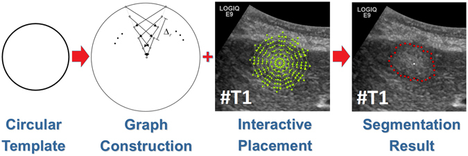
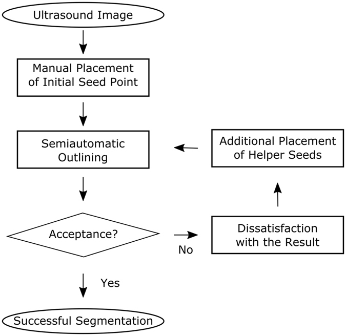
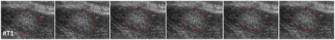
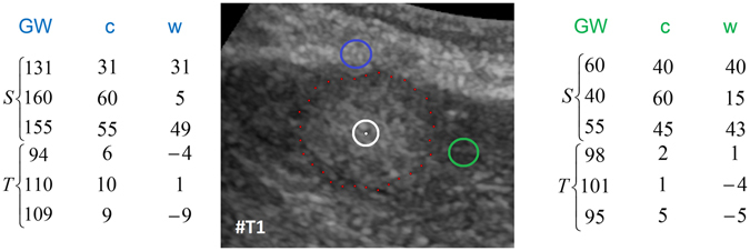
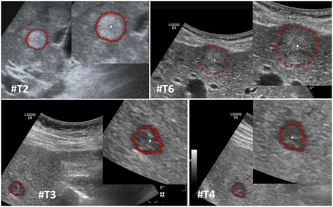
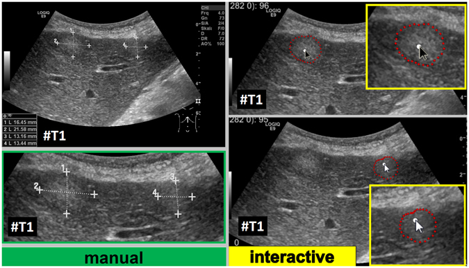
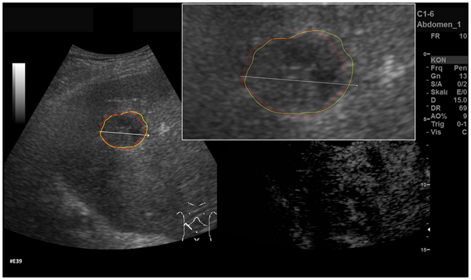
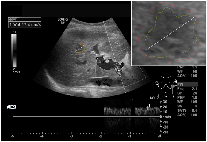
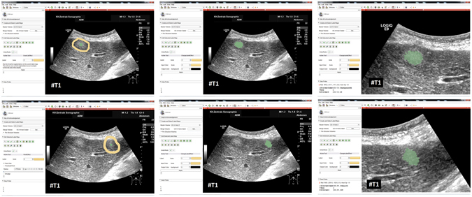
Ultrasound (US) is the most commonly used liver imaging modality worldwide. Due to its low cost, it is increasingly used in the follow-up of cancer patients with metastases localized in the liver. In this contribution, we present the results of an interactive segmentation approach for liver metastases in US acquisitions. A (semi-) automatic segmentation is still very challenging because of the low image quality and the low contrast between the metastasis and the surrounding liver tissue. Thus, the state of the art in clinical practice is still manual measurement and outlining of the metastases in the US images. We tackle the problem by providing an interactive segmentation approach providing real-time feedback of the segmentation results. The approach has been evaluated with typical US acquisitions from the clinical routine, and the datasets consisted of pancreatic cancer metastases. Even for difficult cases, satisfying segmentations results could be achieved because of the interactive real-time behavior of the approach. In total, 40 clinical images have been evaluated with our method by comparing the results against manual ground truth segmentations. This evaluation yielded to an average Dice Score of 85% and an average Hausdorff Distance of 13 pixels.

Figure 1

Different echo pattern of homogenous liver masses in ultrasound B-mode presented in a schematic overview. Relative to the liver echopattern, liver masses can appear hyperechoic (brighter) (A), isoechoic (similar) (B) or hypoechoic (darker) (C). Iso- and hyperechoic liver masses can present with a hypoechoic halo (rim) (D,E). Note: figure adapted from.

Figure 2

Interactive segmentation workflow. Left image: a circular template is used for the underlying graph. Second image from the left: based on the underlying circular template, the graph is constructed. Therefore, rays are sent out radially from the center of the circle template and along these rays the graphs’ nodes are sampled. Afterwards, intra- and inter-edges are established between these nodes (note: the inter-edges depend on a delta value Δ_r). Third image from the left: depending on the interactive placement of the mouse cursor by the user (which is also the center of the circle template/graph), the complete graph (green) is constructed at this position in the ultrasound image. Rightmost image: after the graph cut, the segmentation result (red) is displayed to the user. Note: figure adapted from.

Figure 3

Flow chart of the semi-automatic segmentation approach.

Figure 4

Underlying principle of the graph construction for the interactive segmentation: The upper image shows how the nodes for the graph are sampled. Rays are distributed radially clockwise around a fixed point. Along these rays, the nodes (0, 1, …) are sampled. Bottom images: The intra-edges are constructed within the single rays (an example for two rays is shown in the leftmost image). The next step is to construct the inter-edges between the rays under the specification of the delta value Δ_r: for a delta value Δ_r of zero (Δ_r = 0), only inter-edges are allowed that connect nodes on the same “level” along the rays (see image in the middle). For a delta value Δ_r of one (Δ_r = 1), inter-edges are allowed that connect nodes on different “levels” along the rays, however, only with a maximum “level” distance of one (see rightmost image). Note: the delta values can also be higher, e.g., 2, 3 and so on. Note: figure adapted from.

Figure 5

Segmentation results for different delta values: Δ_r = 0 (leftmost) to Δ_r = 5 (rightmost). Note, the user-defined seed point in white remains for all segmentations at the same position.

Figure 6

Principle of generating the weighted edges between the nodes and the source/sink with an average gray value (for this example 100) sampled around the user-defined seed point (white) in the area of the white circle (US image in the middle). The example on the left belongs to nodes that have been sampled along a ray that runs into a brighter area (blue circle). The example on the right belongs to nodes that have been sampled along a ray that runs into a darker area (green circle). GW are the underlying gray values and the costs c are absolute values between the average gray value (100) and the sampled values behind the nodes (e.g. |100–131| = 31, |100–160| = 60). Finally, the weights w that are assigned to an edge between a sampled node and the source or sink is calculated between two adjacent absolute cost values, e.g. 10–9 = 1. The signs (negative/positive) define if a node is bound to the source or the sink, except for the very first and last nodes (31, 9, 40 and 5), which are bound with their absolute weight values to the source (−9, −5) or sink (31, 40), respectively.

Figure 7

Segmentation results (manual/interactive) of a hyperechoic appearing metastasis with a hypoechoic halo (metastasis of a colon cancer), where the metastasis shows a very low contrast to the surrounding liver parenchyma. The native image with a zoomed view of the metastasis is presented in the left image. A manual measurement of the maximal metastasis diameter (white dotted line between two white crosses) is shown in the middle image. Finally, the rightmost image presents the interactive segmentation results (red dots) with the corresponding user-defined seed point (white). Note: figure adapted from.

Figure 8

Segmentation results for different liver metastases (red dots). Presented are a hyperechoic metastasis of a neuroendocrine neoplasm of the pancreas (upper left), an isoechoic metastasis of a colon cancer (upper right) and two different views of a hypoechoic metastasis of an uveal melanoma (lower images). The white dots in the images are the user-defined seed points. At this positions the user stopped the interactive segmentation, because (s)her was satisfied with the automatic segmentation of the metastasis border. Note: figure adapted from.

Figure 9

Several screenshots from a video where two metastases of a colon cancer in one image were segmented interactively (from the top to the bottom). The upper image presents the native acquisition. The next image presents the position of the mouse cursor where the user started the interactive segmentation. The third image presents the first segmentation result (red dots) at the position of the mouse cursor. In the following image, the user moved the mouse and therefore the seed point (white dot) for the segmentation slightly to the right to get a better segmentation. After being satisfied with the segmentation of the first metastasis, the user moved the mouse to the second metastasis on the right. As seen in the screenshots of the video, the resulting segmentation contours (red dots) collapsed, because in this area, no metastasis is present (note: the screenshots present only a fraction of the whole video). When the user reached the second metastasis on the right, the red segmentation contour automatically expanded again and adapted to the metastasis border (lower two images). The lower image presents the final outlining of the second metastasis where the user stopped the interactive segmentation process.

Figure 10

Direct side-by-side comparison of the interactive segmentation results for the two colon cancer liver metastases from Fig. 9 (right side) and a manual expert measurement of the metastasis (left side). Note: figure adapted from.

Figure 11

Comparison of manual and semi-automated segmentation of a pancreatic cancer liver metastasis. The native image with a zoomed view of the metastasis is presented (white box). The red outline represents the manual segmentation including the white arrow representing the manually drawn maximum diameter. The yellow line represents the result of the semi-automatic segmentation.

Figure 12

Example of a segmentation with a DSC of less than 80%. Depicted is the native image with a zoomed view of the metastasis (white box). The red outline represent the manual segmentation including the white arrow representing the manually drawn maximum diameter. The yellow outline represents the result of the semi-automatic segmentation.

Figure 13

Example of a segmentation with a DSC of less than 80%. Depicted is the native image with a zoomed view of the metastasis (white box). The red outline represent the manual segmentation including the white arrow representing the manually drawn maximum diameter. The yellow outline represents the result of the semi-automatic segmentation.

Figure 14

GrowCut segmentation results for the two metastases from Fig. 9. The left images show the manual initialization of GrowCut: the metastases were initialized with green, and the backgrounds were initialized with yellow. The images in the middle show the segmentation results of GrowCut (green). The right images show a closer view of the segmentation results (green) with a lower opacity.

Figure 15

GrowCut segmentation results for a pancreas metastasis. Equivalent to Fig. 14, the left image shows the manual initialization of GrowCut: the pancreas metastasis was initialized with green, and the background was initialized with yellow. The image in the middle shows the segmentation result of GrowCut (green). The right image shows a closer view of the segmentation result (green) with a lower opacity (0.6).

Figure 16

Direct comparison of our approach with GrowCut (green) for case 39. The red outline represents the manual segmentation including the white arrow representing the manually drawn maximum diameter. The yellow line represents the result of the semi-automatic segmentation (see also Fig. 11). Compared with the manual segmentation, our semi-automatic segmentation algorithm could achieve a DSC of 92.47%. However, compared with the manual segmentation, the GrowCut-based segmentation achieved a DSC of 85.46%.

References

1. Floriani I, et al. Performance of imaging modalities in diagnosis of liver metastases from colorectal cancer: a systematic review and meta-analysis. J Magn Reson Imaging 2010 Jan. 2010;31(1):19–31. - PubMed
1. Seufferlein T, et al. ESMO Guidelines Working Group. Pancreatic adenocarcinoma: ESMO-ESDO Clinical Practice Guidelines for diagnosis, treatment and follow-up. Ann Oncol. Suppl. 2012;7:vii33–40. - PubMed
1. Harvey CJ, Albrecht T. Ultrasound of focal liver lesions. Eur Radiol. 2001;11(9):1578–93. doi: 10.1007/s003300101002. - DOI - PubMed
1. Hohmann J, et al. Characterisation of focal liver lesions with unenhanced and contrast enhanced low MI real time ultrasound: on-site unblinded versus off-site blinded reading. Eur J Radiol. 2012;81(3):e317–24. doi: 10.1016/j.ejrad.2011.10.015. - DOI - PubMed
1. Boen, D. Segmenting 2D Ultrasound Images using Seeded Region Growing. University of British Columbia, Department of Electrical and Computer Engineering, Vancouver, British Columbia, 1–11 (2006).
Publication types