Towards a theory of cortical columns: From spiking neurons to interacting neural populations of finite size

Abstract

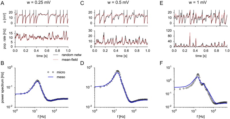
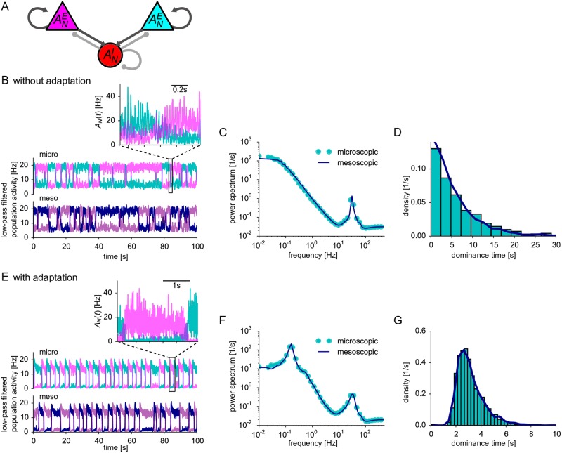
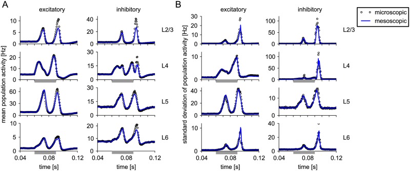
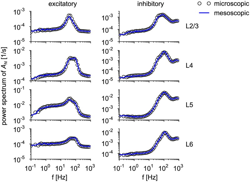
Neural population equations such as neural mass or field models are widely used to study brain activity on a large scale. However, the relation of these models to the properties of single neurons is unclear. Here we derive an equation for several interacting populations at the mesoscopic scale starting from a microscopic model of randomly connected generalized integrate-and-fire neuron models. Each population consists of 50-2000 neurons of the same type but different populations account for different neuron types. The stochastic population equations that we find reveal how spike-history effects in single-neuron dynamics such as refractoriness and adaptation interact with finite-size fluctuations on the population level. Efficient integration of the stochastic mesoscopic equations reproduces the statistical behavior of the population activities obtained from microscopic simulations of a full spiking neural network model. The theory describes nonlinear emergent dynamics such as finite-size-induced stochastic transitions in multistable networks and synchronization in balanced networks of excitatory and inhibitory neurons. The mesoscopic equations are employed to rapidly integrate a model of a cortical microcircuit consisting of eight neuron types, which allows us to predict spontaneous population activities as well as evoked responses to thalamic input. Our theory establishes a general framework for modeling finite-size neural population dynamics based on single cell and synapse parameters and offers an efficient approach to analyzing cortical circuits and computations.

Fig 1. Illustration of population models on the microscopic and mesoscopic level.

(A) Cortical column model [5] with ∼ 80’000 neurons organized into four layers (L2/3, L4, L5, L6) each consisting of an excitatory (“e”) and an inhibitory (“i”) population. On the microscopic level, each individual neuron is described by a generalized integrate-and-fire (GIF) model with membrane potential $u_i^{\alpha }\left(t\right)$, dynamic threshold ${\vartheta }_i^{\alpha }\left(t\right)$ and conditional intensity $f^{\alpha }(u_i^{\alpha }\left(t\right)-{\vartheta }_i^{\alpha }\left(t\right))$. Inset: GIF dynamics for a specific neuron i of population L4e (α = L4e). The neuron receives spikes from neurons in L4e, L4i and L6e, which drive the membrane potential $u_i^{\alpha }\left(t\right)$. Spikes are elicited stochastically by a conditional intensity ${\lambda }_i^{\alpha }\left(t\right)=f^{\alpha }(u_i^{\alpha }\left(t\right)-{\vartheta }_i^{\alpha }\left(t\right))$ that depends on the instantaneous difference between $u_i^{\alpha }\left(t\right)$ and the dynamic threshold ${\vartheta }_i^{\alpha }\left(t\right)$. Spike feedback (voltage reset and spike-triggered threshold movement) gives rise to spike history effects like refractoriness and adaptation. (B) Spike raster plot of the first 200 neurons of each population. The panels correspond to the populations in (A). Layer 4 and 6 are stimulated by a step current during the interval (0.06s, 0.09s) mimicking thalamic input (gray bars). Solid lines show the population activities $A_N^{\alpha }\left(t\right)$ computed with temporal resolution Δt = 0.5 ms, cf. Eq (2). The activities are stochastic due to the finite population size. (C) On the mesoscopic level, the model reduces to a network of 8 populations, each represented by its population activity $A_N^{\alpha }\left(t\right)$. Inset: The mesoscopic model generates realizations of $A_N^{\alpha }\left(t\right)$ from an expected rate ${\overline{A}}^{\alpha }\left(t\right)$, which is a deterministic functional of the past population activities. (D) A corresponding simulation of the mesoscopic model yields population activities with the same temporal statistics as in (B).

Fig 2. How fluctuations of the refractory density effect the population activity.

(A) The conditional intensity ${\lambda }_A\left(t\right|\widehat{t})$ shown as a function of $\widehat{t}$ (left) and t (right). Typically, the conditional intensity increases as the time since the last spike grows and the neuron recovers from refractoriness. (B) For N → ∞, the population activity A(t) (hatched bin) results from ${\lambda }_A\left(t\right|\widehat{t})$ averaged over the last spike times $\widehat{t}$ with a weighting factor $S\left(t\right|\widehat{t})A\left(\widehat{t}\right)$ (blue) corresponding to the density of last spike times. Here, $S\left(t\right|\widehat{t})$ is the survival probability. (C) The last spike times $\widehat{t}$ are discretized into time bins. In the bin immediately before t, a large fluctuation (blue peak) was induced by forcing some of the neurons with last spike time around t* to fire. At time t, the density of last spike times (blue) has a hole and a peak of equal probability mass. The red line shows the pseudo-density $S_0\left(t\right|\widehat{t})A\left(\widehat{t}\right)$ that would be obtained if we had used the survival probability $S_0\left(t\right|\widehat{t})$ of the unperturbed system. The peak at $\widehat{t}=t-\Delta t$ does not contribute to the activity A(t) because of refractoriness, but the hole at $\widehat{t}=t^{*}$ contributes with a non-vanishing rate (A), implying a reduction of A(t) (hatched bin). (D) For a finite population size (here N = 400), the refractory density $S_N\left(t\right|\widehat{t})A_N\left(\widehat{t}\right)$ (blue), determines the expectation $\overline{A}\left(t\right)$ (hatched bin) of the fluctuating activity A_N(t). Analogous to the forced fluctuation in (C), the finite-size fluctuations are associated with negative and positive deviations in the refractory density (holes and overshoots) compared to the non-normalized density $S\left(t\right|\widehat{t})A_N\left(\widehat{t}\right)$ (red line) that would be obtained if only the mean $S\left(t\right|\widehat{t})$ and not the exact survival fraction $S_N\left(t\right|\widehat{t})$ had been taken into account. The variance of the deviations is proportional to $v(t,\widehat{t})$ given by Eq (12). As a function of $\widehat{t}$, $v(t,\widehat{t})$ shows the range of $\widehat{t}$ where deviations are most prominent (bottom). (E, F) Given the number of neurons firing in the bin $[\widehat{t},\widehat{t}+\Delta t)$, $\Delta n\left(\widehat{t}\right)$, the fraction of neurons that survive until time t is shown for ten realizations (gray lines, one highlighted in black for clarity). The mean fraction equals the survival probability $S\left(t\right|\widehat{t})$ (red line, top panel). The variance of the number of survived neurons at time t, $v(t,\widehat{t})N\Delta t$, is shown at the bottom (red line: semi-analytic theory, Eq (12); circles: simulation). (E) $\Delta n\left(\widehat{t}\right)=5$, (F) $\Delta n\left(\widehat{t}\right)=40$.

Fig 3. Population activity of uncoupled leaky integrate-and-fire neurons without adaptation.

(A) Neurons were stimulated by a step current I_ext(t) such that μ = u_rest + RI_ext(t) increased from μ = 15 mV to μ = 30 mV (top). Voltage trace of one of 500 neurons (bottom). Stationary firing statistics (rate and coefficient of variation (CV) of the interspike intervals) corresponding to the two stimuli are indicated above the step current. (B) Realizations of the population activity A_N(t) for the microscopic (top) and mesoscopic (bottom, blue line) simulation. The magenta line shows the expected population rate $\overline{A}\left(t\right)$ given the past actual realization A_N(t′) for t′ < t. (C) The power spectrum of the stationary activity A_N(t) obtained from renewal theory, Eq (134), (black solid line) and from the mesoscopic simulation (blue circles). The top and bottom panel corresponds to weak (μ = 15 mV) and strong (μ = 30 mV) constant stimulation (transient removed).

Fig 4. Population dynamics captures adaptation and burstiness.

(A) 500 adapting leaky integrate-and-fire neurons were stimulated by a step current I_ext that increased μ = u_rest + RI_ext(t) from μ = 12 mV to μ = 27 mV (top). Voltage trace of one neuron (bottom). Stationary firing statistics (rate and coefficient of variation (CV)) corresponding to the two stimuli are indicated above the step current. (B) Realizations of the population activity obtained from microscopic simulation (black) and mesoscopic population equation (blue) as well as $\overline{A}\left(t\right)$ (magenta). (C) Power spectra corresponding to the stationary activity (averaged over 1024 trials each of 20 s length) at low and high firing rates as in (A), circles and lines depict microscopic and mesoscopic case, respectively. Parameters in (A)–(C): u_th = 10 mV, u_r = 25 mV, threshold kernel $\theta \left(t\right)={\sum }_{\ell =1,2}(J_{\theta ,\ell }/{\tau }_{\theta ,\ell })e^{-t/{\tau }_{\theta ,\ell }}$ for t ≥ t_ref with J_θ,1 = 1.5 mV⋅s, τ_θ,1 = 0.01 s, J_θ,2 = 1.5 mV⋅s, τ_θ,2 = 1 s. (D) Bursty neuron model. (i) Biphasic threshold kernel θ(t), where a combination of a negative part (facilitation) and a positive part (adaptation) yields a bursty spike pattern, (ii) sample firing pattern of one neuron. (iii) The interspike interval distribution with values of rate and CV. (E) Power spectrum of the population activity A_N(t) shown in (D)-(iv). Parameters in (D) and (E): μ = 20, u_th = 10 mV, u_r = 0 mV, τ_m = 0.01 s, facilitation: J_θ,1 = −0.45 mV⋅s, τ_θ,1 = 0.05 s; adaptation: J_θ,2 = 2.5 mV⋅s, τ_θ,2 = 1 s.

Fig 5. Mesoscopic dynamics of E-I network for varying network size N, connection probability p and number of synapses per neuron C.

(A) Left: Schematic of the network of N^E excitatory and N^I = N^E/4 inhibitory leaky integrate-and-fire (LIF) neurons, each receiving C^E = pN^E (C^I = pN^I) connections from a random subset of excitatory (inhibitory) neurons. Total numbers are N = N^E + N^I and C = C^E + C^I. At C = 200, the synaptic strength is w = 0.3 mV and −gw = −1.5 mV for excitatory and inhibitory connections, respectively. To preserve a constant mean synaptic input, the synaptic strength is scaled such that Cw = const‥ Right: Schematic of a corresponding mesoscopic model of two interacting populations. (B) Trajectories of u(t) for five example neurons (top) and of the excitatory population activity $A_N^E\left(t\right)$ obtained from the network simulation (middle) and the mesoscopic simulation (bottom, dark green) for C = N = 50; time resolution Δt = 0.2 ms. The light green trajectory (bottom panel) depicts the expected population activity ${\overline{A}}^E\left(t\right)$ given the past activity. (C) Power spectra of $A_N^E\left(t\right)$ for different network sizes while keeping p = 1 fixed (microscopic: symbols, mesoscopic: solid lines with corresponding dark colors). (D) Sample trajectories corresponding to the green curve in (E) (N = 1000, p = 0.2). (E) Analogously to (C) but varying the connection probabilities while keeping C = pN = 200 fixed. (F) Sample trajectories corresponding to the green curve in (G) (N = 200, C = 40). (G) Analogously to (C) but varying the number of synapses C while keeping N = 200 fixed. Note that the mesoscopic theory (black solid line) is independent of C because the product Cw, which determines the interaction strength in the mesoscopic model (see, left panel of (A)), is kept constant. Parameters: μ^E/I = 24 mV, ${\Delta }_u^{E/I}=2.5$ mV and θ^E/I(t) ≡ 0 (no adaptation).

Fig 6. Mean-field approximation of synaptic input for randomly connected networks.

The same E-I network as in Fig 5 with N = 500 neurons and connection probability p = 0.2 was simulated for increasing synaptic strength w^EE = w^IE = w (w^EI = w^II = −5w) of excitatory (inhibitory) connections: (A, B) w = 0.25 mV, (C, D) w = 0.5 mV (E, F) w = 1 mV. (A, C, E) Top: Membrane potential of one example neuron shows fluctuations due to spike input from C = 100 presynaptic neurons (black line), which represent a random subset of all 500 neurons. The mean-field approximation of the membrane potential (dashed red line) assumes that the neuron had the same firing times but was driven by all neurons, i.e. by the population activities $A_N^E\left(t\right)$ and $A_N^I\left(t\right)$, with rescaled synaptic strength $w_{\text{MF}}^{E/I}=p{w}^{E/I}$. Although individual membrane potentials differ significantly from the mean-field approximation (top), the relevant population-averaged hazard rates ${\overline{A}}_{\text{micro}}^{E/I}\left(t\right)\equiv \frac{1}{N^{E/I}}{\sum }_{i=1}^{N^{E/I}}\lambda \left(t\right|{\widehat{t}}_i)$ (bottom) are well predicted by the mean-field approximation. (B, D, F) Corresponding power spectra of the (excitatory) population activity for microscopic (circles) and mesoscopic (blue solid line) simulation. Parameters as in Fig 5 except μ^E/I = 18 mV.

Fig 7. Finite-size induced switching in a bistable network.

(A) Schematic of a winner-take-all network architecture: Two competing excitatory populations (N^E1 = N^E2 = 400) interact with a common inhibitory population (N^I = 200). (B)-(D) In the absence of adaptation (θ^E/I(t) ≡ 0), the excitatory populations switch between low and high activities in an irregular fashion (B). Activities in (B, E) are low-pass-filtered by a moving average of 100 ms. Top: full network simulation. Inset: Magnified view of the activities for 1 s (without moving average) showing fast large-amplitude oscillations. Bottom: mesoscopic simulation. (C) The power spectrum of the activity of the excitatory populations exhibits large low-frequency power and a high-frequency peak corresponding to the slow stochastic switching between high- and low-activity states and the fast oscillations, respectively. (D) The density of the dominance times (i.e. the residence time in the high-activity states) has an exponential form. (E-G) Like (B-D) but excitatory neurons exhibit weak and slow adaptation (${\theta }^E\left(t\right)=(J_{\theta }/{\tau }_{\theta })e^{-t/{\tau }_{\theta }}$ with J_θ = 0.1 mV⋅s, τ_θ = 1 s for t ≥ t_ref). Switching between high- and low-activity states is more regular than in the non-adapting case as revealed by a low-frequency peak in the power spectrum (F) and a narrow, unimodal density of dominance times (G). In (C, D) and (F, G) microscopic and mesoscopic simulation correspond to cyan symbols/bars and dark blue solid lines, respectively. Parameters: μ^E/I = 36 mV except for μ^E = 36.5 in (E-G) to compensate adaptation. Time step Δt = 0.01 ms (microscopic), Δt = 0.2 ms (mesoscopic). Efficacies of excitatory and inhibitory connections: w^E = 0.0624 mV and w^I = −0.2496 mV (B-D), and w^E = 0.096 mV and w^I = −0.384 mV (E-G), p = 1, ${\Delta }_u^{E/I}=2.5$ mV.

Fig 8. Time-dependent statistics of the population activities in a cortical column model.

(A) Trial-averaged population activities (peri-stimulus-time histogram, PSTH) in the modified Potjans-Diesmann model as illustrated for a single trial in Fig 1. Circles and blue solid line show microscopic simulation (250 trials, simulation time step Δt = 0.01 ms) and mesoscopic simulation (1000 trials, Δt = 0.5 ms), respectively. A step current mimicking thalamic input is provided to neurons in layer 4 and 6 during a time window of 30 ms as indicated by the gray bar. Rows correspond to the layers L2/3, L4, L5 and L6, respectively, as indicated. Columns correspond to excitatory and inhibitory populations, respectively. (B) Corresponding, time-dependent standard deviation of A_N(t) measured with temporal resolution Δt = 0.5 ms.

Fig 9. Stationary statistics of population activities in a cortical column model.

Power spectra of the spontaneous population activities A_N(t) in the modified Potjans-Diesmann model in the absence of time-dependent thalamic input (corresponding to the activities shown in Fig 1B (microscopic) and Fig 1D (mesoscopic) outside of the stimulation window. Circles and blue solid lines represent microscopic and mesoscopic simulation, respectively. Rows correspond to the layers L2/3, L4, L5 and L6, respectively, as indicated. Columns correspond to excitatory and inhibitory populations, respectively.

Fig 10. Different interpretations of the function m(t,t^) (red line).

(A) As a function of $\widehat{t}$ (or as a function of k in discrete time), m(t_l, t_k) represents the distribution of last spike times ${\widehat{t}}_i$ across the population at time t = t_l. (B) As a function of time t (or as a function of the index l in discrete time), m(t_l, t_k) represents the survival number, i.e. the number of neurons which fired in the interval [t_k, t_k + Δt) which survived (did not fire) until time t = t_l. The activity Δn(t_k), i.e. the number of neurons that fired in the k-th time bin, is depicted by a blue line. The population size is N = 1000.

Fig 11. Pseudocode for the integration of the mesoscopic population equation.

Note that procedure UpdatePopulation in line 12 is shown in Fig 12.

Fig 12. Pseudocode for the update of the variables of a given population.

Note that the adaptation kernel θ_k′ ≡ θ((K − k′)Δt), the quasi-renewal kernel ${\tilde{\theta }}_{k^{\prime }}\equiv \tilde{\theta }\left(\right(K-k^{\prime })\Delta t)/N$, Eq (33), as well as the exponentials $e^{-\frac{\Delta t}{{\tau }_{\text{m}}}}$ and $J_{\theta ,\ell }{e}^{-K\Delta t/{\tau }_{\theta ,\ell }}$ can be precomputed.

References

1. Wang Y, Toledo-Rodriguez M, Gupta A, Wu C, Silberberg G, Luo J, et al. Anatomical, physiological and molecular properties of Martinotti cells in the somatosensory cortex of the juvenile rat. J Physiol. 2004;561(1):65–90. 10.1113/jphysiol.2004.073353 - DOI - PMC - PubMed
1. Sugino K, Hempel CM, Miller MN, Hattox AM, Shapiro P, Wu C, et al. Molecular taxonomy of major neuronal classes in the adult mouse forebrain. Nat Neurosci. 2006;9(1):99–107. 10.1038/nn1618 - DOI - PubMed
1. Lefort S, Tomm C, Sarria JCF, Petersen CCH. The excitatory neuronal network of the C2 barrel column in mouse primary somatosensory cortex. Neuron. 2009;61(2):301–316. 10.1016/j.neuron.2008.12.020 - DOI - PubMed
1. Harris KD, Shepherd GMG. The neocortical circuit: themes and variations. Nat Neurosci. 2015;18(2):170–181. 10.1038/nn.3917 - DOI - PMC - PubMed
1. Potjans TC, Diesmann M. The cell-type specific cortical microcircuit: relating structure and activity in a full-scale spiking network model. Cereb Cortex. 2014;24(3):785–806. 10.1093/cercor/bhs358 - DOI - PMC - PubMed
LinkOut - more resources