Hybrid finite difference/finite element immersed boundary method

Abstract

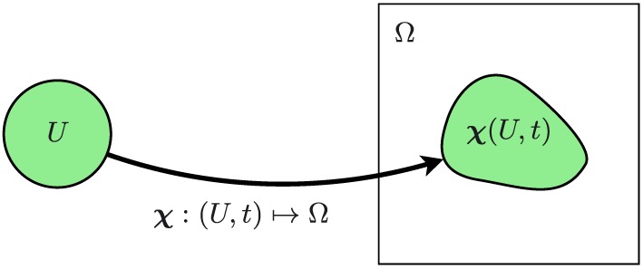
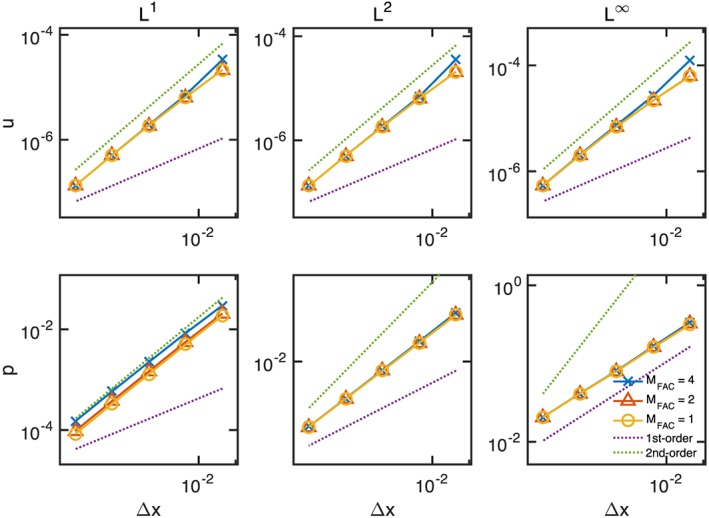
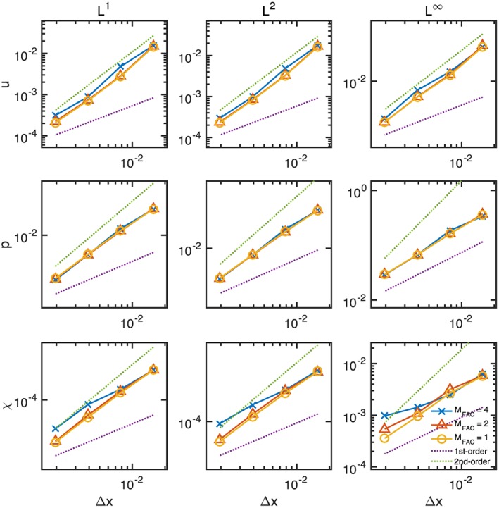
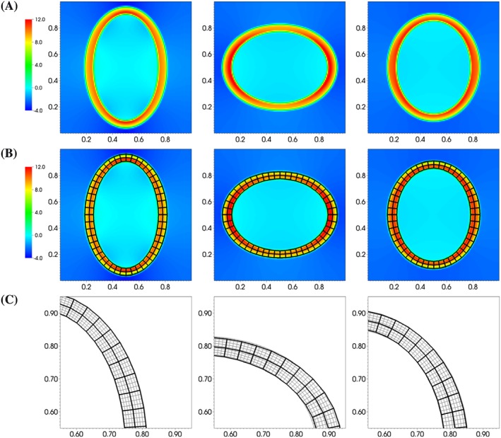
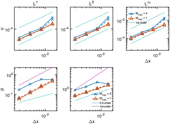
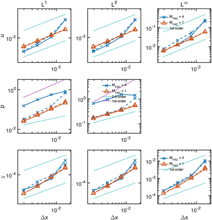
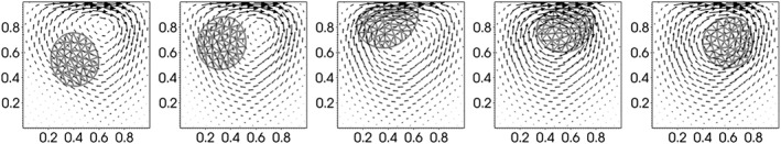
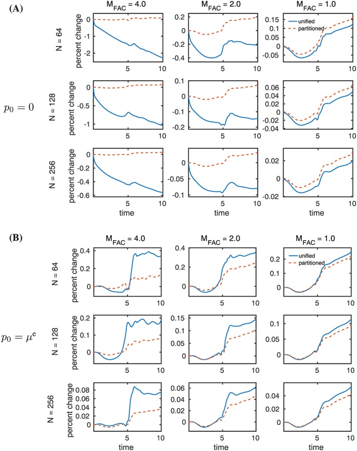
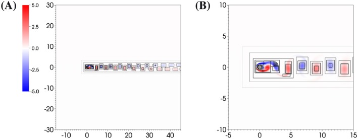
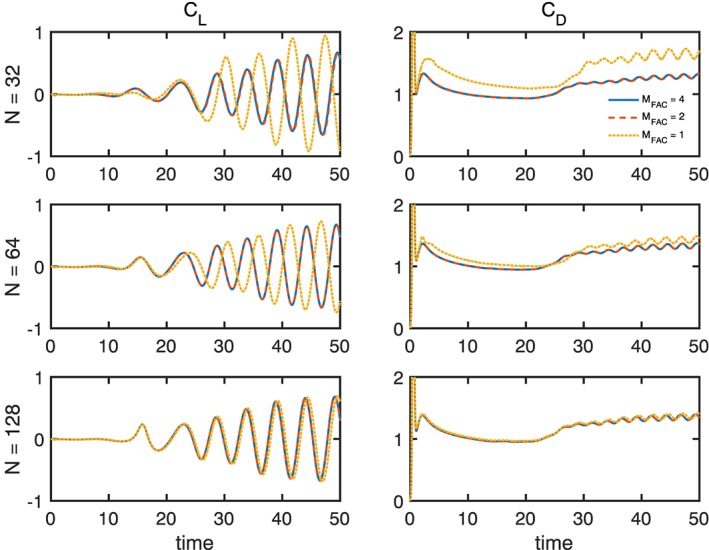
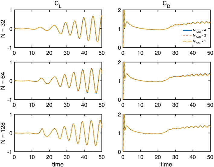
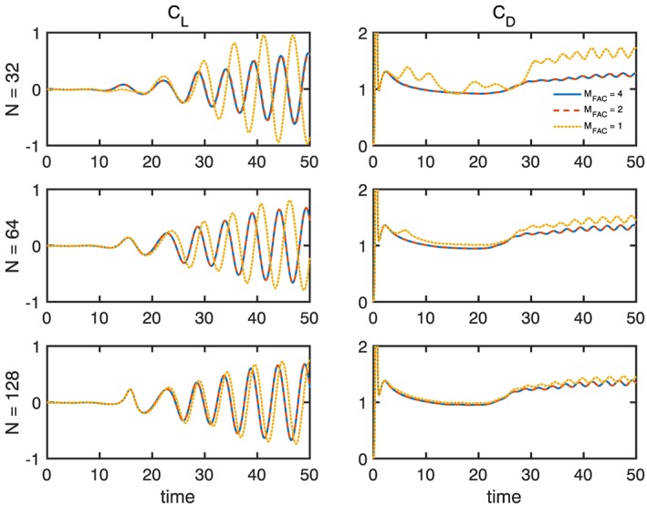
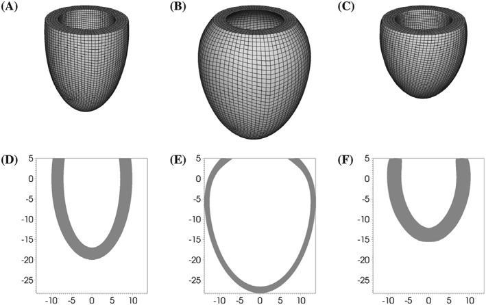
The immersed boundary method is an approach to fluid-structure interaction that uses a Lagrangian description of the structural deformations, stresses, and forces along with an Eulerian description of the momentum, viscosity, and incompressibility of the fluid-structure system. The original immersed boundary methods described immersed elastic structures using systems of flexible fibers, and even now, most immersed boundary methods still require Lagrangian meshes that are finer than the Eulerian grid. This work introduces a coupling scheme for the immersed boundary method to link the Lagrangian and Eulerian variables that facilitates independent spatial discretizations for the structure and background grid. This approach uses a finite element discretization of the structure while retaining a finite difference scheme for the Eulerian variables. We apply this method to benchmark problems involving elastic, rigid, and actively contracting structures, including an idealized model of the left ventricle of the heart. Our tests include cases in which, for a fixed Eulerian grid spacing, coarser Lagrangian structural meshes yield discretization errors that are as much as several orders of magnitude smaller than errors obtained using finer structural meshes. The Lagrangian-Eulerian coupling approach developed in this work enables the effective use of these coarse structural meshes with the immersed boundary method. This work also contrasts two different weak forms of the equations, one of which is demonstrated to be more effective for the coarse structural discretizations facilitated by our coupling approach.

Keywords: finite difference method; finite element method; fluid-structure interaction; immersed boundary method; incompressible elasticity; incompressible flow.

Figure 1

Lagrangian and Eulerian coordinate systems. The Lagrangian material coordinate domain is U, and the Eulerian physical coordinate domain is Ω. The physical position of material point X at time t is χ(X,t), the physical region occupied by the structure is χ(U,t), and the physical region occupied by the fluid is Ω\χ(U,t)

Figure 2

Schematic of the staggered‐grid layout of Eulerian degrees of freedom in 2 spatial dimensions. The pressures are approximated at cell centers, indicated by (i,j), the x ₁‐components of the velocity and force are approximated on the x ₁‐edges, $(i-\frac{1}{2},j)$ or $(i+\frac{1}{2},j)$, and the x ₂‐components of the velocity and force are approximated on the x ₂‐edges, $(i,j-\frac{1}{2})$ or $(i,j+\frac{1}{2})$

Figure 3

Prolonging the elastic force density from the Lagrangian mesh onto the Eulerian grid. Starting with an approximation to the force density at the nodes of the Lagrangian mesh A, we use the interpolatory FE basis functions to determine the force density at interaction points that are defined by a quadrature rule B, and then spread those forces from the interaction points to the background Eulerian grid using the smoothed delta function δ _h(x) C. This approach permits Lagrangian meshes that are significantly coarser than the Eulerian grid so long as the “net” of interaction points is sufficiently dense. Denser nets of interaction points can be obtained, for instance, by increasing the order of the numerical quadrature scheme

Figure 4

Representative results from the dynamic (γ=0.15) version of the idealized anisotropic shell model of Section 5.1.1 for N=128 over the time interval 0⩽t⩽0.75. The computed pressure and structure deformation for M _fac=4 are shown in A and B. The computed deformations obtained with M _fac=1 and M _fac=4 are compared in C. The coarse and fine structural meshes yield essentially identical kinematics

Figure 5

Errors in u and p in L ¹, L ², and $L^{\infty }$ norms for the static (γ=0) version of the idealized anisotropic shell model of Section 5.1.1. Reference lines with slopes of ‐1 and ‐2 are also shown. The velocity converges at second‐order accuracy in all norms, whereas the pressure converges at second‐order in the L ¹ norm, at first‐order in the $L^{\infty }$ norm, and at order 1.5 in the L ² norm

Figure 6

Errors in u, p, and χ in L ¹, L ², and $L^{\infty }$ norms for the dynamic (γ=0.15) version of the idealized anisotropic shell model of Section 5.1.1. Reference lines with slopes of ‐1 and ‐2 are also shown. The velocity converges at second‐order accuracy in all norms, whereas the pressure converges at second‐order in the L ¹ norm, at first‐order in the $L^{\infty }$ norm, and at order 1.5 in the L ² norm. The displacement converges at essentially second‐order rates in the L ¹ and L ² norms, and at a slightly lower rate in the $L^{\infty }$ norm

Figure 7

Similar to Figure 4, but here, showing results obtained using the orthotropic shell model of Section 5.1.2 for N=128 and the partitioned (split) weak formulation over the time interval 0⩽t⩽1.25. As in Figure 4, the coarse and fine structural meshes yield very similar kinematics

Figure 8

Errors in uand p in L ¹, L ², and $L^{\infty }$ norms for the static (γ=0) version of the orthotropic shell model of Section 5.1.2. Errors for the unified formulation appear as solid lines, and errors for the partitioned formulation appear as dashed lines. Reference lines with slope ‐1 are provided for the u error data. For p, reference lines with slopes ‐1 and ‐0.5 are provided for the L ¹ and L ² norm data, respectively. Because this test includes discontinuities in the pressure at fluid‐structure interfaces, the present method does not yield convergence in p in the $L^{\infty }$ norm. The partitioned formulation generally yields improved accuracy compared to the unified formulation, especially for the pressure for relatively coarse structural mesh spacings

Figure 9

Errors in u, p, and χ in L ¹, L ², and $L^{\infty }$ norms for the dynamic (γ=0.15) version of the orthotropic shell model of Section 5.1.2. Errors for the unified formulation appear as solid lines, and errors for the partitioned formulation appear as dashed lines. Reference lines with slope ‐1 are provided for the u and χ error data. For p, reference lines with slopes ‐1 and ‐0.5 are provided for the L ¹ and L ² norm data, respectively. The unified formulation generally yields modest improvements in the accuracy for u and χ, whereas the partitioned formulation generally yields improved accuracy for p, especially for relatively coarse structural mesh spacings.

Figure 10

A soft neo‐Hookean disc in a lid‐driven cavity flow using the partitioned (split) weak formulation withN=128 and M _fac=4 over the time interval 3⩽t⩽7

Figure 11

Percent change in structure volume for the soft elastic disc benchmark of Section 5.2 as a function of time using Equation (65) with A, p ₀=0 and B, p ₀=μ ^e. Results are shown for Cartesian grids of size N=64, 128, and 256 with relative Lagrangian mesh spacings M _fac=4, 2, and 1. The amount of spurious volume change converges to zero at first order. At coarser relative mesh spacings, the partitioned (split) formulation yields substantially better volume (area in 2 spatial dimensions) conservation than the unified (unsplit) formulation. Volume conservation is substantially improved for the unified formulation by setting p ₀=μ ^e. The volume change is less than 0.4% for all cases considered except for the unified formulation with p ₀=0 and M _fac=4.

Figure 12

Vortices shed from a stationary circular cylinder at R e=200. This computation uses a six‐level locally refined grid with a refinement ratio of two between levels and an N×N coarse grid with N=128. Regions of local mesh refinement are indicated by rectangular boxes, with lighter grey boxes indicating coarser levels of refinement and black boxes indicating the finest regions of the locally refined grid. A, The full computational domain and B, a magnified view of the flow field near the cylinder

Figure 13

Lift (C _L) and drag (C _D) coefficients for flow past a stationary cylinder at R e=200. The computational domain Ω is discretized using a six‐level locally refined grid with a refinement ratio of two between levels and an N×N coarse grid. The spacing between the nodes of the immersed structure is approximately M _facΔx _finest. Under simultaneous Lagrangian and Eulerian grid refinement, the scheme converges to the same dynamics for all values of M _fac. Notice, however, that the best accuracy is obtained for larger values of M _fac. Using a relatively finer structural mesh spacing results in larger lift and drag coefficients and lower vortex shedding frequencies. Thus, smaller values of M _fac increase the effective numerical size of the cylinder

Figure 14

Similar to Figures 13 and 15, but here, using a 3‐point kernel function.71 Unlike the case of the 4‐  and 6‐point kernels, comparable accuracy is obtained for all values of M _fac considered

Figure 15

Similar to Figures 13 and 14, but here, using a six‐point kernel function with higher continuity order.72 As with the four‐point kernel, the best accuracy is obtained for larger values of M _fac. In this case, however, using relatively fine structural mesh spacings yields erratic results on coarser Eulerian grids (eg, M _fac=1 for N=32)

Figure 16

Inflation and active contraction of an idealized model of the left ventricle of the heart. A, The reference configuration of the left ventricle model is a truncated ellipsoid. B, Passive inflation of an isotropic version of the left ventricular model. C, Active contraction of a transversely isotropic left ventricle model that includes transmural fiber rotation. Notice the torsion induced by the active contractile forces. D‐F, Slices of the configurations shown in panels A to C

Figure 17

Circumferential, longitudinal, and transverse strains along the endocardium, epicardium, and midwall in the idealized left ventricle model for A, passive inflation and B, active contraction. Strains are plotted at selected points running from apex to base. See Land et al45 for additional details on the positions of the sample points. The computed strains are in excellent agreement (within 1% with consensus results obtained by other structural mechanics codes using the same model45

Figure 18

Difference in the displacement of the actively contracting fiber‐reinforced left ventricle model using different N×N×N Cartesian grids. A, Distribution of difference in the structural displacement obtained using N=48 and N=64. B, Distribution of difference in the structural displacement obtained using N=64 and N=96

Figure 19

Fiber strain distribution in the actively contracting fiber‐reinforced left ventricle model obtained using a 64×64×64 Cartesian grid

References

1. Peskin CS. Flow patterns around heart valves: a numerical method. J Comput Phys. 1972;10(2):252‐271.
1. Peskin CS. Numerical analysis of blood flow in the heart. J Comput Phys. 1977;25(3):220‐252.
1. Peskin CS. The immersed boundary method. Acta Numer. 2002;11:479‐517.
1. Miller LA, Peskin CS. When vortices stick: an aerodynamic transition in tiny insect flight. J Exp Biol. 2004;207(17):3073‐3088. - PubMed
1. Miller LA, Peskin CS. A computational fluid dynamics of ‘clap and fling’ in the smallest insects. J Exp Biol. 2005;208(2):195‐212. - PubMed
Publication types