Population assessment using multivariate time-series analysis: A case study of rockfishes in Puget Sound

Abstract

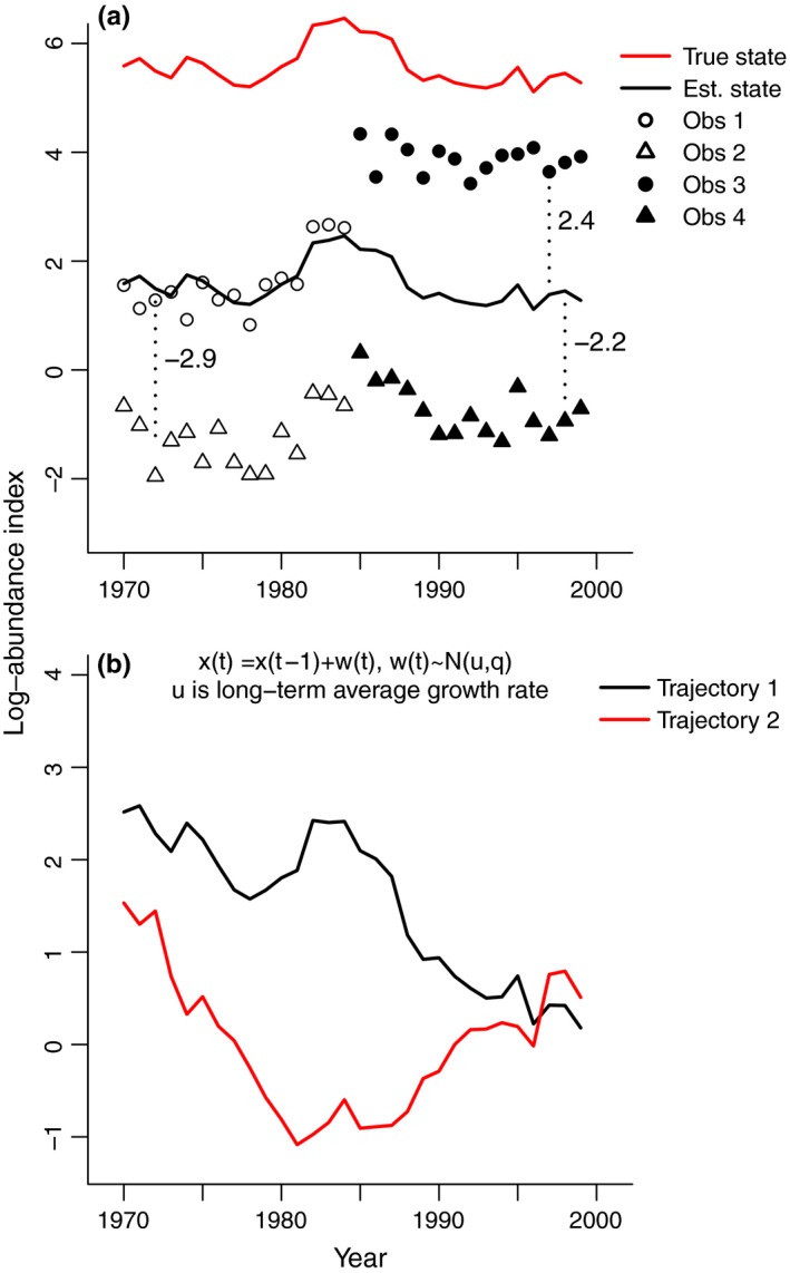
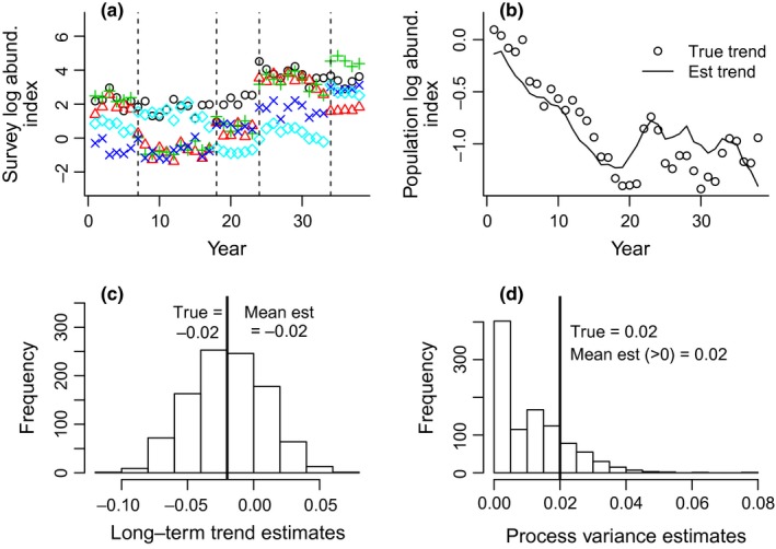
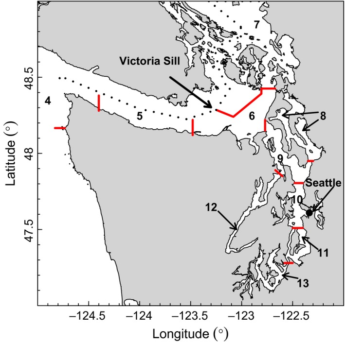
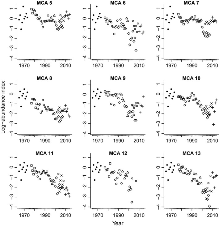
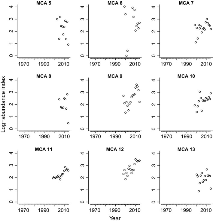
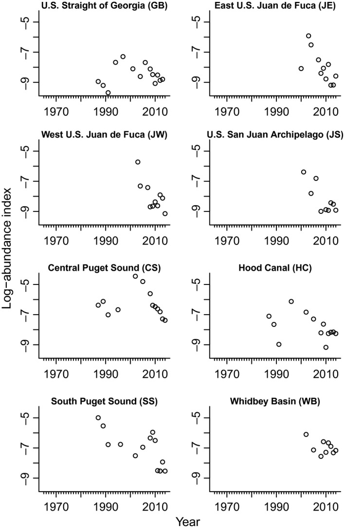
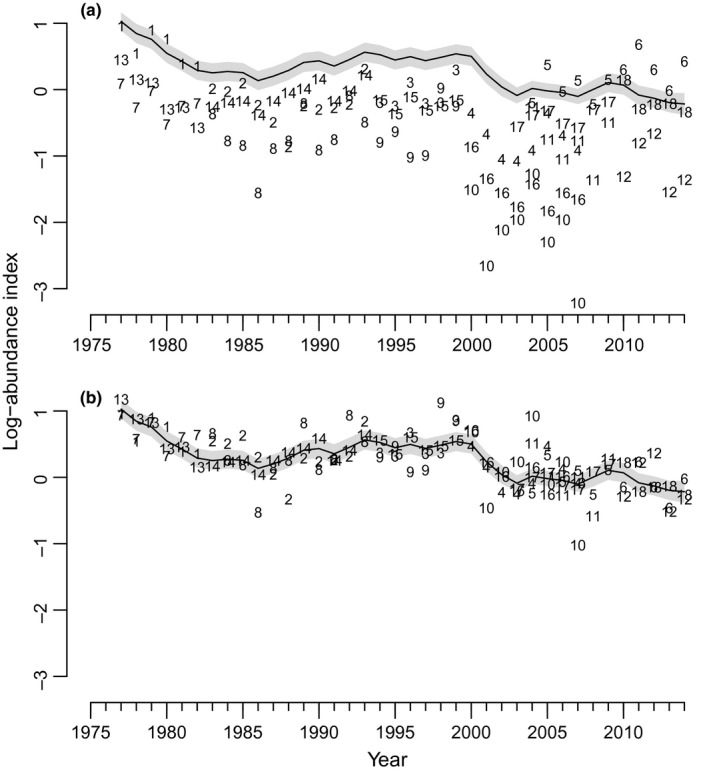
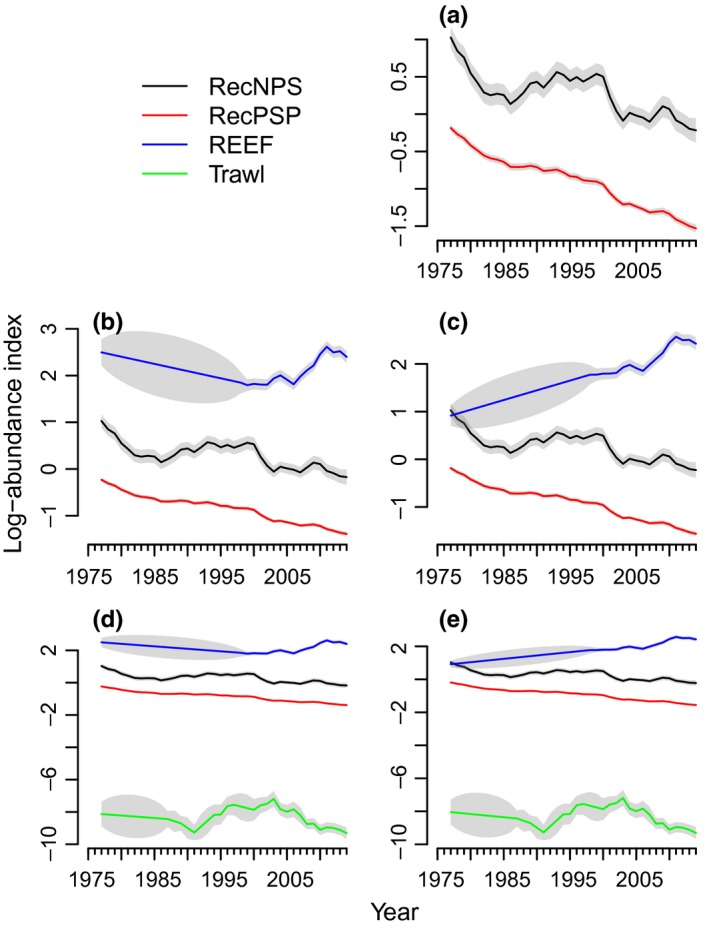
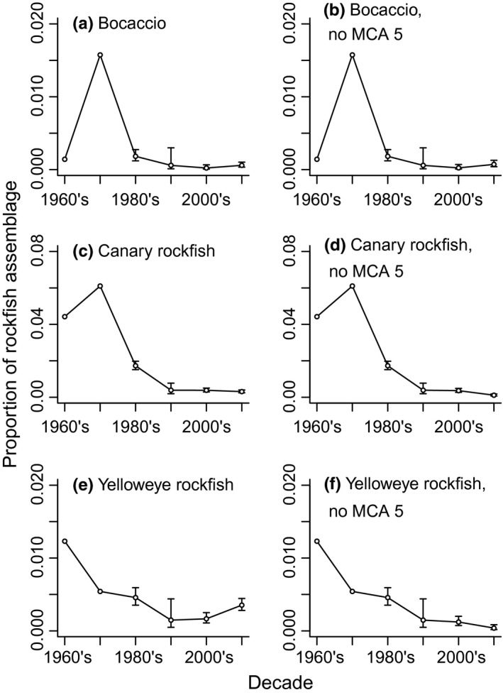
Estimating a population's growth rate and year-to-year variance is a key component of population viability analysis (PVA). However, standard PVA methods require time series of counts obtained using consistent survey methods over many years. In addition, it can be difficult to separate observation and process variance, which is critical for PVA. Time-series analysis performed with multivariate autoregressive state-space (MARSS) models is a flexible statistical framework that allows one to address many of these limitations. MARSS models allow one to combine surveys with different gears and across different sites for estimation of PVA parameters, and to implement replication, which reduces the variance-separation problem and maximizes informational input for mean trend estimation. Even data that are fragmented with unknown error levels can be accommodated. We present a practical case study that illustrates MARSS analysis steps: data choice, model set-up, model selection, and parameter estimation. Our case study is an analysis of the long-term trends of rockfish in Puget Sound, Washington, based on citizen science scuba surveys, a fishery-independent trawl survey, and recreational fishery surveys affected by bag-limit reductions. The best-supported models indicated that the recreational and trawl surveys tracked different, temporally independent assemblages that declined at similar rates (an average of -3.8% to -3.9% per year). The scuba survey tracked a separate increasing and temporally independent assemblage (an average of 4.1% per year). Three rockfishes (bocaccio, canary, and yelloweye) are listed in Puget Sound under the US Endangered Species Act (ESA). These species are associated with deep water, which the recreational and trawl surveys sample better than the scuba survey. All three ESA-listed rockfishes declined as a proportion of recreational catch between the 1970s and 2010s, suggesting that they experienced similar or more severe reductions in abundance than the 3.8-3.9% per year declines that were estimated for rockfish populations sampled by the recreational and trawl surveys.

Keywords: Endangered Species Act; Sebastes; data‐limited; multivariate autoregressive state‐space models; population viability analysis; risk assessment; rockfishes; trend analysis.

Figure 1

Illustration of the structure of a multivariate autoregressive state‐space (MARSS)‐based population viability analysis (PVA). (a) Four surveys (Obs 1–4) with one true population trajectory (red line) and an estimated trajectory (scaled estimate, black line). The true population trajectory is “hidden” (i.e., not directly observable). The four different time series (surveys) follow the hidden population trajectory but with different scaling because each is a somewhat different index survey. Numbers on the figure indicate a (scaling up or down) for the survey data. Only three of the scaling factors can be estimated. One scaling factor is set to zero and the estimate for the population trajectory is scaled to that survey. The scaling factors for the other surveys can be estimated because they are all assumed to be observing the same population (black line). Although estimation is improved if the segments overlap, the model can still estimate the black line, and parameters associated with it, when there are gaps between segments as long as the segments are not too short. Replication by way of multiple observations at different sites or with different surveys can enhance the ability of the model to estimate population trajectory substantially. (b) An example of a MARSS model with the same long‐term population growth rate u but two different trajectories (states) which covary

Figure 2

Results of the simulation study of estimation of the population growth and process error for data structured similar to the Recreational Fishery (Rec) survey in the North Puget Sound (NPS). The data are divided into segments of 6, 11, 6, 10, and 5 years long. There are three spatial replicates [marine catch areas (MCAs)]. In this simulation, there is one population trajectory representing the rockfish assemblage surveyed by the Rec survey in NPS. The true population is declining 2.0% per year on average in the simulation; process variance was set to 0.02. For this simulation, the scaling factors were chosen to increase with each successive segment, creating the illusion of an increasing trend. One thousand datasets and population trajectories were generated; long‐term population growth rate and process variance were estimated for each. (a) Example of the true population trajectory and estimated population trajectory for one dataset. (b) Histogram of the 1000 long‐term population growth rate estimates showing that they are unbiased (i.e., non‐zero). (c) Histogram of the process variance estimates. A feature of state‐space models is that there can be a likelihood maximum with one of the variances at zero (degenerate model). The interior (non‐zero) variance estimates are unbiased. In practice, if a degenerate estimate occurs, one examines the likelihood surface to find the interior local maximum where all variances are non‐zero

Figure 3

Marine catch areas (MCAs) for Washington Department of Fish and Wildlife (WDFW) recreational catch data. Data from North Puget Sound [(NPS) MCAs 5–7] and Puget Sound Proper [PSP (MCAs 8–13)] were used in the analyses. The major regional water masses are NPS (MCAs 5–7), Whidbey Basin (MCA 8), Main Basin (MCAs 9–11, 13), and Hood Canal (MCA 12). The dashed line indicates the US.–Canadian border. Red lines indicate MCA boundaries

Figure 4

Log‐abundance index from the Washington Department of Fish and Wildlife (WDFW) recreational survey. The data are the log of catch (retained and released) per angler effort (catch‐per‐unit effort, (CPUE), where effort is defined as one angler trip. The different symbols represent periods with different bag limits. Note that the + and × are data obtained using a new methodology that includes a phone survey in addition to a creel (dockside) survey. The new methodology yields CPUE values that are higher than the prior method (see overlapping years with open diamonds and ×)

Figure 5

Reef Environmental Education Foundation (REEF) survey data used in the MARSS analysis by Washington marine catch areas (MCA). North Puget Sound (NPS) = MCAs 5–7; Puget Sound Proper (PSP) = MCAs 8–13. The data do not include young‐of‐year or Puget Sound Rockfish S. emphaeus

Figure 6

Washington Department of Fish and Wildlife (WDFW) trawl survey catch‐per‐unit effort [CPUE (number per km²)] by trawl area. GB = US Strait of Georgia, JE = east US Juan de Fuca, JW = west US Juan de Fuca, JS = San Juan Islands, HC = Hood Canal, CS = central Puget Sound, SS = South Puget Sound, WI = Whidbey Island Basin. GB, JE, JW, and JS comprise North Puget Sound (NPS). CS, HC, WI, and SS comprise Puget Sound Proper (PSP)

Figure 7

Estimated trajectory (solid line) for total rockfish in North Puget Sound [NPS (Rec_NPS)] from the best‐supported model using the Rec data only showing the effect of the scaling parameter a. Numbers refer to separate Rec time‐series for each regulatory period in marine catch areas (MCAs) 5–7. (a) Raw data for each NPS time‐series, and (b) data for each NPS time‐series corrected by the scaling parameter a. Grey envelopes indicate 95% confidence intervals

Figure 8

Estimated trajectories for total rockfish based on the best‐supported models. (a) Recreational Fishery Survey (Rec) data only: one u, two states, u _GPS = −0.038. (b) Rec + REEF data: one u, three states, u _GPS = −0.031. (c) Rec + REEF data: two u’s, three states, u _Rec = −0.039, u _REEF = 0.041. (d) Rec + REEF + Trawl data: two u's, four states, u _Rec/Trawl = −0.039, u _REEF = 0.041. (e) Rec + REEF + Trawl data: one u, four states, u _GPS = −0.032. Grey envelopes indicate 95% confidence intervals

Figure 9

Prevalence of bocaccio, canary, and yelloweye rockfishes as a proportion of the total rockfish assemblage in the Washington Department of Fish and Wildlife (WDFW) recreational Survey for marine catch areas (MCAs) 5‐13 or 6‐13. a) bocaccio MCAs 5‐13, b) bocaccio MCAs 6‐13, c) canary rockfish MCAs 5‐15, d) canary rockfish MCAs 6‐13, e) yelloweye rockfish MCAs 5‐13, f) yelloweye rockfish MCAs 6‐13. MCA 5 is closest to the coast in the Strait of Juan de Fuca and is not included in the population designation for the listed species. Error bars indicate 95% confidence limits. Data are shown in Table S11.

References

-
- Agresti, A. , & Coull, B. A. (1998). Approximate is better than “exact” for interval estimation of binomial proportions. American Statistician, 52, 119–126.
- Ahrestani, F. S. , Hebblewhite, M. , & Post, E. (2013). The importance of observation versus process error in analyses of global ungulate populations. Scientific Reports, DOI: 10.1038/srep03125 - DOI - PMC - PubMed
- Andelman, S. J. , Groves, C. , & Regan, H. M. (2004). A review of protocols for selecting species at risk in the con‐ text of US Forest Service viability assessments. Acta Oecologica, 26, 75–83.
- Anderson, L. E. , Lee, S. T. , & Levin, P. S. (2013). Costs of delaying conservations: Regulations and recreational values of exploited and co‐occurring species. Land Economics, 89, 371–385.
LinkOut - more resources
Full Text Sources
Other Literature Sources
Miscellaneous