Quantifying Golgi structure using EM: combining volume-SEM and stereology for higher throughput

Abstract

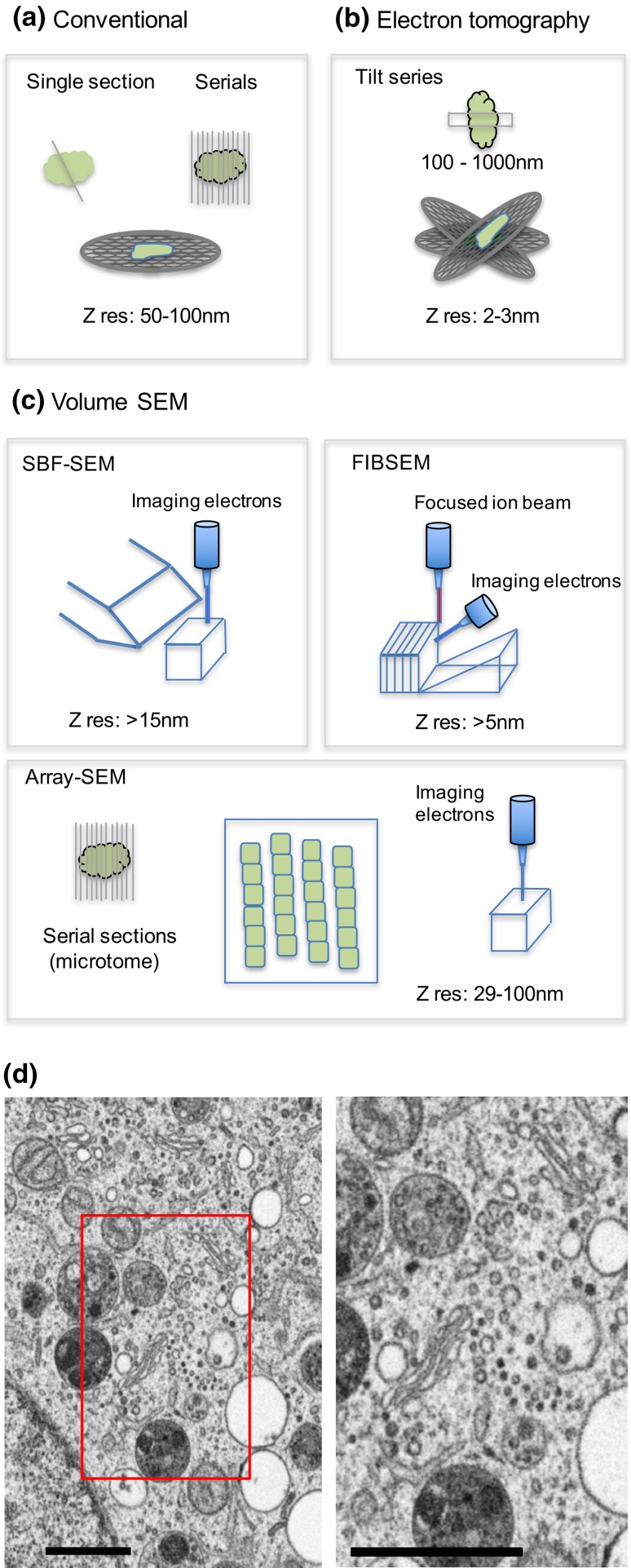
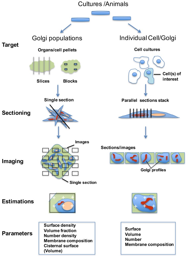
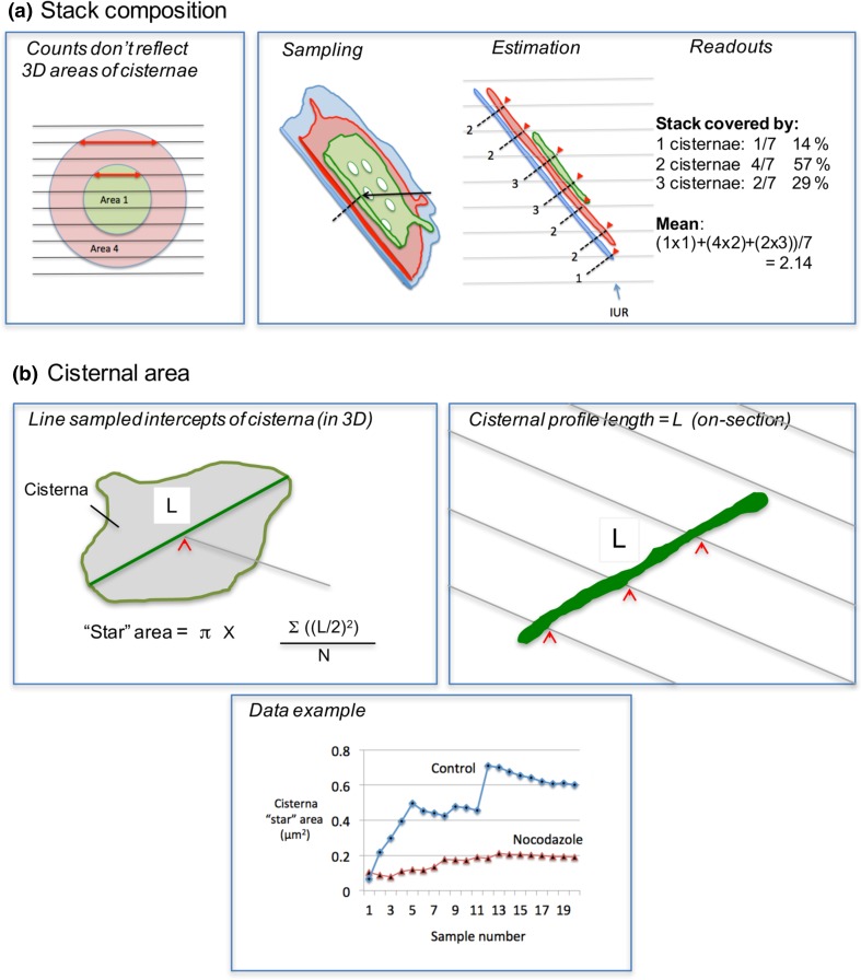
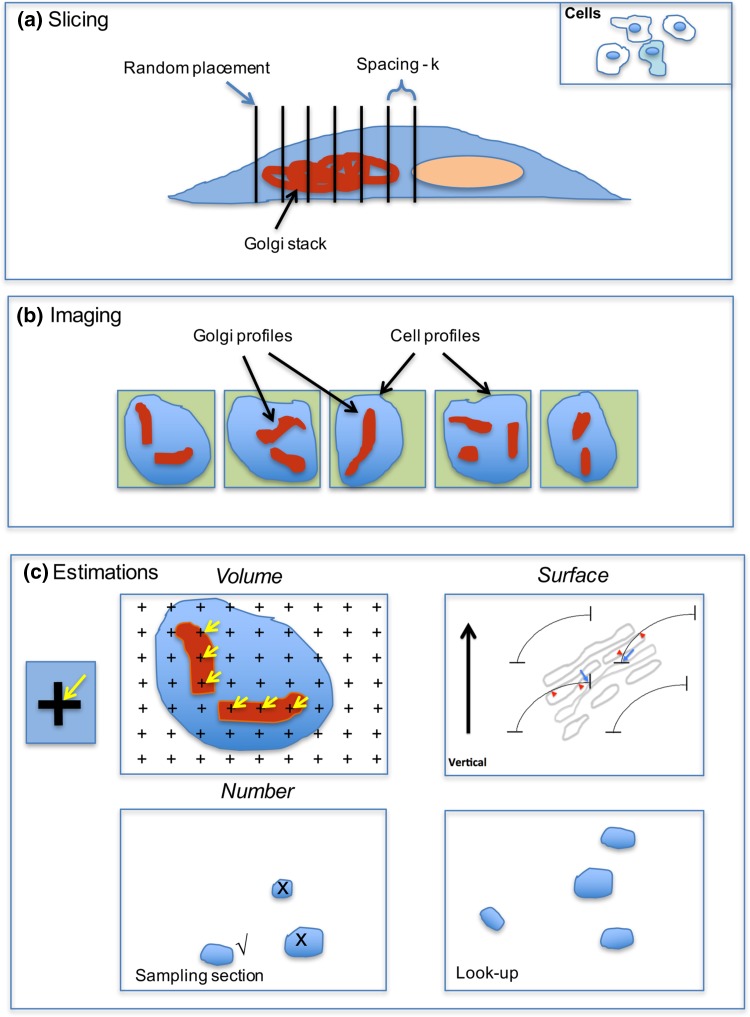
Investigating organelles such as the Golgi complex depends increasingly on high-throughput quantitative morphological analyses from multiple experimental or genetic conditions. Light microscopy (LM) has been an effective tool for screening but fails to reveal fine details of Golgi structures such as vesicles, tubules and cisternae. Electron microscopy (EM) has sufficient resolution but traditional transmission EM (TEM) methods are slow and inefficient. Newer volume scanning EM (volume-SEM) methods now have the potential to speed up 3D analysis by automated sectioning and imaging. However, they produce large arrays of sections and/or images, which require labour-intensive 3D reconstruction for quantitation on limited cell numbers. Here, we show that the information storage, digital waste and workload involved in using volume-SEM can be reduced substantially using sampling-based stereology. Using the Golgi as an example, we describe how Golgi populations can be sensed quantitatively using single random slices and how accurate quantitative structural data on Golgi organelles of individual cells can be obtained using only 5-10 sections/images taken from a volume-SEM series (thereby sensing population parameters and cell-cell variability). The approach will be useful in techniques such as correlative LM and EM (CLEM) where small samples of cells are treated and where there may be variable responses. For Golgi study, we outline a series of stereological estimators that are suited to these analyses and suggest workflows, which have the potential to enhance the speed and relevance of data acquisition in volume-SEM.

Keywords: FIBSEM; Golgi; Quantification; SBF-SEM; Sampling; Stereology; Volume-SEM.

Fig. 1

New volume-SEM techniques compared to conventional and tomographic TEM analysis. Using conventional techniques comprehensive 3D information has been acquired using either serial sections (a 50-100 nm thickness) or electron tomography (b z resolution as little as 2–3 nm). Tomography involves tilting of thicker samples (200-1000nm; Lindsay and Ellisman, 1985; Walther et al. 2013) and back projection to provide 3D information (Donohoe et al. ; Marsh and Pavelka ; Marsh et al. 2004). However, the usefulness of tomography for whole Golgi studies has been limited due to the comparatively shallow sample depth and narrow scale. These serial section/imaging techniques are labour intensive in obtaining full 3D datasets of Golgi. Volume-SEM techniques (c) automate collection of exhaustive serial section/images and include serial block face (SBF-SEM) and focused ion beam SEM (FIBSEM) and array-SEM. SBF-SEM and FIBSEM improve z resolution with section/imaging thickness between 5 and 30 nm and work by iterative removal of sample block-face by physical slicing (SBF-SEM) or by ion beam erosion (FIBSEM), followed by imaging in the SEM. Improved z resolution yields large datasets requiring storage in silico, and prompts development and unbiased data mining using stereology. SBF-SEM techniques are adapted to imaging wider scales of tissue (Bosch et al. ; Kuwajima et al. ; Titze and Genoud 2016), while FIBSEM is narrow-scale allowing focused analysis on single cells. Imaging the block-face improves stability of the 3D array. Array-SEM involves preparation of large arrays of serial sections on conventional microtomes, and section thickness can be little as 29 nm (Kasthuri et al. 2015). Typically, sections are collected on tapes, which are mounted in short series on hard supports prior to SEM imaging. Sections can be prone to dimensional instability and folding. In this case sections can be re-probed reducing the need for in silico storage. d Illustrates a typical image from of a Golgi complex region of a HeLa cells obtained using FIBSEM imaging (5 nm pixels). Boxed area in low magnification image (left) is displayed at higher magnification (right). Bars 1 µM

Fig. 2

Sampling strategies allowing the use of single sections or parallel section stacks. The population may comprise animals, cell cultures or subcellular Golgi fractions from which organs or cell/organelle pellets or culture dishes are processed for fixation. Left Single section analysis on Golgi populations. The items (organs/cell pellets) are fragmented or sliced systematic uniform random (SUR) before being further divided to provide specimen blocks. For single section analysis, blocks are most conveniently sectioned by microtomy (inside the SEM (SBF-SEM) or on a conventional microtome, (array-SEM) before imaging using SEM). Typically, 10–20 images are taken in an SUR array. Estimations are carried out using geometric probes applied to the images (see Figs. 3, 4, 5). Right parallel section stacks on Golgi from single cells of interest. Randomly selected dishes and randomly selected cells from subpopulations of interest (e.g. those obtained using CLEM) are identified before, during or after processing for SEM. Golgi complexes of interest are relocated, and a randomly placed section stack with equal spacing is generated through the organelle. Images of the entire Golgi structure are probed using estimators for volume, surface and number on all sections of the stack (Fig. 6). The sampling intensity (5–10 sections) not only provides useful precision on individual cells/Golgi but also increases the number of cells that can be analysed, as compared to exhaustive serial section/image analysis (see text)

Fig. 3

Estimation of volume and surface from single sections. a The packing density of structure volume in a reference volume (e.g. cytoplasm) can be estimated by counting the ratio of points that fall on structure (Golgi component of interest) versus the points that fall on the reference volume (e.g. cytoplasm). Points are defined by the corners that lie between grid-lines or crosses arranged in a regular lattice pattern. b The packing density of surface in a reference volume is estimated using interactions between randomly positioned and oriented test lines and Golgi membranes. Sample position is randomised using SUR sampling and orientation randomised using the isector [embedding in a ball of gelatin, which is rolled randomly before slicing; Nyengaard and Gundersen ; isotropic uniform random (IUR) section]. Systematic arrays of test lines are superimposed on images and intersection counts (I) between line edges and Golgi membranes counted (red arrowheads). Surface density, Sv = 2I/L, where line length L applied to the reference space (e.g. Golgi stack) is estimated by counting points over Golgi cisternae (blue arrows) multiplied by the line length associated with each point. c In the vertical section (VS) method, a section is cut in a vertical direction, orthogonal to a convenient/arbitrary horizontal plane such as the bottom of a culture dish. The section must have random placement and freedom of orientation around the vertical. Cycloid arcs aligned with the vertical direction represent a full distribution of isotropic lines in 3D space. Intersections (I; red arrrowheads) are counted and surface density, Sv = 2I/L, where again, L is estimated by point counting (blue arrows) as described in (b). d Local vertical windows (LVWs). In IUR sections, the animal cell Golgi twists and turns in 3D making it difficult to identify and quantify regional elements (e.g. cis, medial and trans). Local vertical windows (LVWs) first “choose” stack profiles with membranes that present clear cisternal membrane profiles with minimal thickness. These represent Golgi stacks sectioned in a cis–trans direction. A line of best fit drawn “parallel” to Golgi cisternae membranes now traces a horizontal plane in 3D (dashed line) with the vertical in a cis–trans direction. A cycloid array is used to estimate the Sv of any membrane or substructure across this axis estimated using the same formula as above (red arrowheads indicate intersections between cycloids and cisternal membranes; point counts for estimating line length omitted for clarity). Graph in (e) compares estimates obtained using LVWs and isotropic line methods. For these data multiple Golgi stacks were generated in RK-13 cells using the drug nocodazole. Estimates obtained with the LVW method stabilized faster than for the isotropic lines method across a series of images. LVWs, N = 12 images and for isotropic line, N = 20. Error bars are standard error of the mean calculated for a ratio estimate according to Cochran (1977). Section orientation requirements: R-sections with random orientations; VS-sections with vertical orientation

Fig. 4

Single section analysis of number and reference volume. Number estimation requires a volume probe composed of two sections with known spacing (a disector). a The principle is to select particle profiles on one plane (sampling section) using an unbiased counting rule applied to a counting frame (quadrat). Particles are selected if enclosed either partially or completely within the frame and are not crossed by the forbidden line (red). Particles are counted only if they disappear in the lookup section (Q ⁻). b In conventional TEM, when the section thickness approaches the diameter of the structures (e.g. for 60-nm COPI vesicles), a single section can be used for counting (the workup checks that the fraction of equatorial profiles generated from one section (red lines) that cannot be identified as such in the next adjacent section). This approach is called a one-section disector. However, care must be exercised when using this approach with volume SEM methods. One problem occurs when SEM imaging comes from surface layer of a much thicker section, so that vesicles waists will be missed (e.g. Array-SEM or SBF-SEM). In this case increasing the imaging depth could solve this problem. Another possibility is that imaging and section thickness are very small compared to the vesicle size (e.g. with FIBSEM) so that the same vesicle waist may appear in multiple sections (thereby decreasing the fraction of vesicle profiles that disappear in adjacent sections). In this case it could be useful to assemble a projection image from a ministack of sections, which itself approximates in thickness to size of the vesicles in question. The numerical density of vesicles (or fenestrations for example) counted in disectors can be related to volume by performing point counting for the appropriate reference space found within the disector (not shown). A systematic lattice of points is applied to the sampling frame and the number hitting the reference space profile is recorded. The estimate of the volume of reference space inside the disector is P × a × h, where P is the sum of points, a is the area associated with one point on the lattice and h is the distance between the section planes used to make the disector. Numerical density is given by Q ⁻/ P × a × h. c The mean volume of a reference component or space (e.g. cell cytoplasm) estimated using a disector; (see a). Structures in the disector (ticks; Q ⁻) and points (P) over the component/space profiles are counted. Mean volume is given by: P × a × h/Q ⁻. Again the second section is prepared parallel to the first and distance between sections (h) is computed. Low-magnification SEM images are used for disector and point counting

Fig. 5

Single sections: specialised estimators. a Composition. Counts of cisternae in sections are a biased measure of relative 3D number (Lucocq and Hacker 2013). A randomly positioned stack of sections hits a larger (red) cisterna eight times and the smaller (green) cisterna four times reflecting the twofold greater height of the large cisterna. By contrast there is a fourfold difference between relative areas of the two cisternae in 3D. This is reported by relative profile length on the sections (red arrows mark the lengths of two sectioned profiles). The composition of the stack “ribbon” can be sensed using SUR test lines with random placement and isotropic uniform random (IUR) orientation. At each intercept the number of cisternae in the stack is counted in a direction orthogonal to the stack (dashed lines). Results are summed from multiple SUR images and provide estimates of proportions of the stack ribbon covered by 1,2,3, etc. cisternae. b Cisternal “spread” or “star” area. Top left Principle: the IUR grey line identifies a randomly positioned intercept (red arrowhead) on the cisternal surface (grey fill). The randomly oriented intercept (green) passes through the sampled point. The length of the intercept is used to compute the area of the surface from the equation. Top right in a real sample (randomised in orientation during embedding), random locations on a cisterna (sectioned profile in green) are located (red arrowheads) using a systematic array of test lines (grey) applied to a section. The length of cisternal profile represents L and is estimated for each random sampling “hit” using the same test system of lines. In the example for each random hit there are three line hits on the green cisterna profile. Each of these hit totals report an estimated cisternal length of π/2 × I × d where I is the number of intersections (3) and d is the real spacing of the test lines (the grid must be randomised in orientation and position relative to the cisternal profile). Notice that this estimator of intercept (cisternal profile) length works for curvilinear profiles. Star area will reflect the degree of connectivity/extent of the cisternae in 3D. Bottom: star areas of Golgi cisternae in RK13 cells with and without fragmentation of the Golgi using the microtubule depolymerising agent nocodazole (sample number indicates the number of SUR images used for each cumulative estimate from this single illustrative experiment)

Fig. 6

Parallel section stacks (Golgi subpopulations/individual cells). The cell(s) of interest is (are) identified (for example, using correlative light and electron microscopy (CLEM)) and prepared for SEM. a and b A stack of 5–10 parallel images is recorded spanning the entire Golgi organelle. The stack is positioned at random and each section evenly spaced by a known interval/section number. In FIBSEM the orientation of the sections is easily set as orthogonal to the horizontal plane of the cell culture dish (vertical section). c Estimations Volume of Golgi structures can be estimated using Cavalieri’s volume estimator V = Σ A × k, where A is the area of sectioned profiles summed over all section planes and k is the spacing of the images. Area A can be computed from P × a, where P is the sum of points (black crosses) hitting the profiles on all the stack images and a, is the area associated with each point on the grid lattice (applied SUR). The estimator is unbiased if section planes used are infinitely thin with respect to the object of interest. Corrections may need to be applied when slice thickness is substantial compared with the spacing k (Howard and Reed 2005). When sections are vertical, the surface density of Golgi component membranes can be estimated using a cycloid arc test system applied along the vertical direction (SURS pattern; see text and Fig. 3). The total surface is obtained by multiplying Sv by reference volume obtained using the Cavalieri estimator. Number can be estimated using at least two sections in close proximity or adjacent to each other in the stack (bottom left and right). Structures that produce profiles in one section, but not the next (√) have edges between the sections and, therefore, are counted (disector principle; Sterio ; Gundersen 1986). The sections need to be spaced at 1/3 to 1/4 of the diameter of the structures counted to make structures easy to follow. For convex objects such as vesicles, counting is straightforward because each object has a single edge (regardless of its size). One of the sections can belong to the section stack used for volume or surface estimation. The total number of structures in the Golgi is estimated from the number of disappearing profiles multiplied by 1/(fraction of sections used for counting) (Gundersen ; Lucocq et al. ; Smythe et al. 1989). For example, if COPI vesicles are counted using ten pairs of adjacent 20-nm sections through a 5-µm Golgi and the distance between the pairs is 50 sections then the estimate of COPI number is vesicle edge counts (Q−) × 50/2 (the denominator is 2 because counting can be done in both directions to improve efficiency). If there are 500–1000 COPI vesicles then 20–40 vesicles will be counted for each cell. If the section thickness approaches the size of the vesicles (as is the case of conventional 50 nm resin sections and 60–70 nm COPI vesicles) a majority of vesicle equators detected in the sampling section may be absent in the lookup section. Under these conditions a single section disector (Lucocq et al. ; Nyengaard and Gundersen 2006) is established and comparison with the lookup section is not necessary, speeding up the analysis. Care must be exercised when designing single section disectors for use with the surface imaging used in volume SEM (see Fig. 4b and text for details). Numerical density can be computed by combining disector counts with point counting or surface estimators. Another possible readout is to relate the number of one structure to another using the ratio of counts (Gundersen 1986)

Fig. 7

Experimental design for stereological estimation on single slices and parallel section series in volume-SEM. Two experimental pathways are outlined here, using either single sections for investigating the parameters of Golgi populations, or randomly placed parallel section stacks for analysis of subpopulations/individual Golgi. The single section approach is more suited to SBF-SEM and array-SEM, because they produce larger section areas than FIBSEM. Here the primary accessible parameters are densities, which may be converted to amounts using estimates of the reference volume (curved arrow). In the case of parallel section stacks, absolute volume and number are directly accessible but surface must be determined as a density first before combining with the volume estimate to derive membrane surface (curved arrow). In either approach volume and number can be determined on sections that are arbitrary, randomly oriented or vertically oriented. Surface density and specialised estimators require isotropic uniform random (IUR) sections or vertical sections (VS; details are given in the text). CIS cisternae, TUB tubules, VES vesicles, CYT cytoplasm, Fenestr fenestrations

References

1. Amos WB, Grimstone AV. Intercisternal material in the Golgi body of Trichomonas. J Cell Biol. 1968;38:466–471. doi: 10.1083/jcb.38.2.466. - DOI - PMC - PubMed
1. Baddeley A, Jensen EBV. Stereology for statisticians. Boca Raton: Chapman and Hall/CRC press; 2004. p. 23.
1. Baddeley AJ, Gundersen HJ, Cruz-Orive L. Estimation of surface area from vertical sections. J Microsc. 1986;142:259–276. doi: 10.1111/j.1365-2818.1986.tb04282.x. - DOI - PubMed
1. Ballerini M, Milani M, Costato M, Squadrini F, Turcu IC. Life science applications of focused ion beams (FIB) Eur J Histochem. 1997;41(Suppl 2):89–90. - PubMed
1. Bannykh SI, Rowe T, Balch WE. The organization of endoplasmic reticulum export complexes. J Cell Biol. 1996;135:19–35. doi: 10.1083/jcb.135.1.19. - DOI - PMC - PubMed
MeSH terms
LinkOut - more resources