

Exploratory adaptation in large random networks
- PMID: 28429717
- PMCID: PMC5413947
- DOI: 10.1038/ncomms14826
Exploratory adaptation in large random networks
Abstract
The capacity of cells and organisms to respond to challenging conditions in a repeatable manner is limited by a finite repertoire of pre-evolved adaptive responses. Beyond this capacity, cells can use exploratory dynamics to cope with a much broader array of conditions. However, the process of adaptation by exploratory dynamics within the lifetime of a cell is not well understood. Here we demonstrate the feasibility of exploratory adaptation in a high-dimensional network model of gene regulation. Exploration is initiated by failure to comply with a constraint and is implemented by random sampling of network configurations. It ceases if and when the network reaches a stable state satisfying the constraint. We find that successful convergence (adaptation) in high dimensions requires outgoing network hubs and is enhanced by their auto-regulation. The ability of these empirically validated features of gene regulatory networks to support exploratory adaptation without fine-tuning, makes it plausible for biological implementation.
Conflict of interest statement
The authors declare no competing financial interests.
Figures
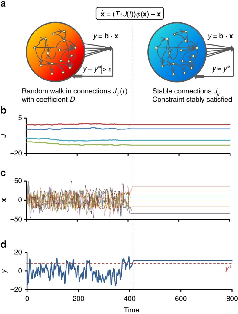
 (y−y*). The random walk stops when the mismatch is stably reduced to zero (right; ‘frozen' regime). (b–d) Example of exploration and convergence. Shown are representative trajectories of connection strengths (b), microscopic variables (c) and the phenotype y (d) before and after convergence to a stable state satisfying the constraint. The network in this example has scale-free (SF) out-degree distribution (a=1, γ=2.4) and Binomial in-degree distribution
  . N=1,000, y*=10, D=10−3, g0=10. See Methods for more details.
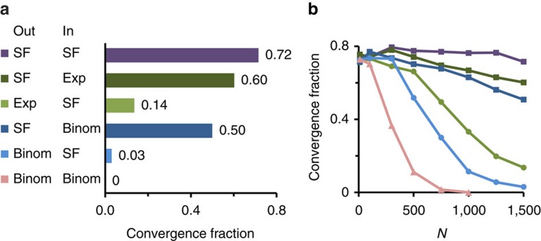
 ; Exp, (β=3.5).
 ; Exp, (β=3.5).
 and N). Other parameters are g0=10, α=100, ɛ=3, c=0.2, D=10−3 and y=0.
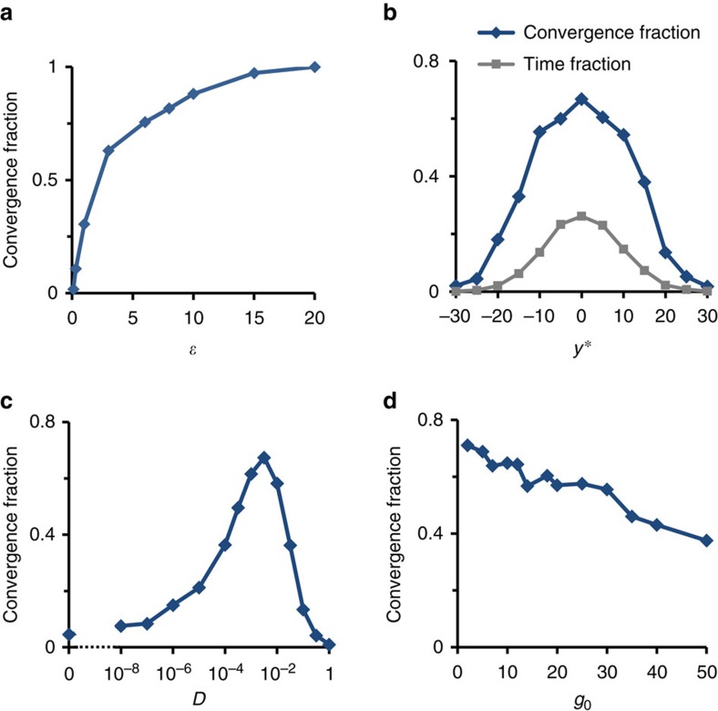
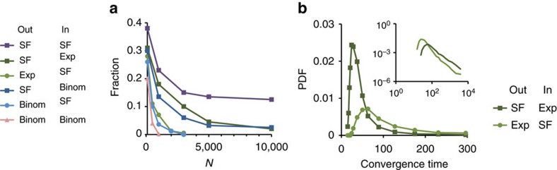
 degree distributions. Unless otherwise specified, all ensembles have N=1,000, y*=0, g0=10, and D=10−3.
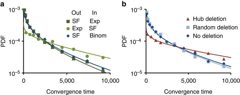
 ; Exp, (
 ).
).
 ; Exp, (
 ).
).References
-
- López-Maury L., Marguerat S. & Bhler J. Tuning gene expression to changing environments: from rapid responses to evolutionary adaptation. Nat. Rev. Genet. 9, 583–593 (2008). - PubMed
-
- Gerhart J. & Kirschner M. Cells, Embryos, and Evolution: Toward a Cellular and Developmental Understanding of Phenotypic Variation and Evolutionary Adaptability Blackwell Science (1997).
-
- Braun E. The unforeseen challenge: from genotype-to-phenotype in cell populations. Rep. Prog. Phys. 78, 036602 (2015). - PubMed
MeSH terms
LinkOut - more resources
Full Text Sources
Other Literature Sources
