Inferring the physical properties of yeast chromatin through Bayesian analysis of whole nucleus simulations

Abstract

Background: The structure and mechanical properties of chromatin impact DNA functions and nuclear architecture but remain poorly understood. In budding yeast, a simple polymer model with minimal sequence-specific constraints and a small number of structural parameters can explain diverse experimental data on nuclear architecture. However, how assumed chromatin properties affect model predictions was not previously systematically investigated.

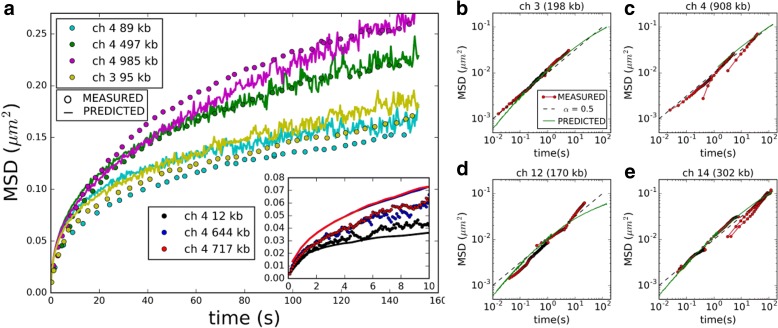
Results: We used hundreds of dynamic chromosome simulations and Bayesian inference to determine chromatin properties consistent with an extensive dataset that includes hundreds of measurements from imaging in fixed and live cells and two Hi-C studies. We place new constraints on average chromatin fiber properties, narrowing down the chromatin compaction to ~53-65 bp/nm and persistence length to ~52-85 nm. These constraints argue against a 20-30 nm fiber as the exclusive chromatin structure in the genome. Our best model provides a much better match to experimental measurements of nuclear architecture and also recapitulates chromatin dynamics measured on multiple loci over long timescales.

Conclusion: This work substantially improves our understanding of yeast chromatin mechanics and chromosome architecture and provides a new analytic framework to infer chromosome properties in other organisms.

Keywords: Chromatin; Chromosomes; Nuclear architecture; Polymer models; Yeast.

Fig. 1

Main components of our computational framework for Bayesian inference of chromatin parameters from whole nucleus simulations. a Simulations: we consider a number n =144 of different parameter values Π_i = (P _i, C _i, W _i, L _i), where P _i is the chromatin persistence length, C _i the chromatin compaction, W _i the chromatin width, and L _i the length of microtubules (see Table 1, Additional file 2). The discretization of the parameter space is illustrated on the left (crosses), highlighting persistence length P and compaction C. Each Π_i defines a separate model M _i = M(Π_i), for which we run two to six independent dynamic simulations of all 16 chromosomes in the nucleus with random initializations. Three-dimensional snapshots are shown for a model with high P and high C (top) and a model with low P and low C (bottom). Each simulation run calculates changes in chromosome configurations over millions of time steps, as illustrated for two time points t ₁ and t _N (only chromosome 4 is shown). By sampling these simulation runs, we predict various observables, $Y_k^{{\mathit{M}}_i}$, such as the average distance $〈{\mathrm{d}}_{\mathit{AB}}^{{\mathit{M}}_i}〉$ between two loci A and B, or the average contact frequencies between chromosomes i and j. b For any value of the parameters Π (within the allowed range), an interpolation scheme calculates the predicted value of the observables Y _k ^M(Π), e.g. 〈d_AB ^Π〉 shown here as a heat map, from the discrete models M _i (crosses). c Experimental data Y _k ^E, such as the average distance between loci A and B measured by imaging, 〈d_AB ^E〉, are compared to the predictions 〈d_AB ^Π〉 for all Π. d, e Similarly, contact frequencies between chromosomes i and j are predicted for all Π (here i=j) (d) and compared to measurements from Hi-C experiments (e). f, g Parameter inference: given an experimental dataset, using the Bayes rule and Markov chain Monte Carlo sampling, we calculate the posterior probability density of any subset of parameters, such as (P, C). Isocontour lines enclose the region of high probability. This can be done for individual experimental data, e.g. 〈d_AB ^E〉 (f), or for a combination of multiple datasets, e.g. mean distances between loci and chromosome contact frequencies (g). The maximum a posteriori estimate of the parameters (MAP) defines a model that provides the best match to the experimental data

Fig. 2

Validation of inference method on simulated data. This figure presents results of our parameter inference method when simulated data are used as input instead of experimental data. a–j Inferred posterior probability densities for chromatin compaction C and persistence length P for data generated by a model with parameters Π₀ = (P ₀, C ₀, W ₀, L ₀) = (41 nm, 50 bp/nm, 45 nm, 300 nm). The blue and red contour lines enclose regions corresponding to 68% and 95% of the probability mass, respectively. The red diamond indicates the true parameter values: (P ₀, C ₀) = (41 nm, 50 bp/nm). The green dot indicates the maximum a posteriori (MAP) estimate, i.e. the parameter values $\left(\widehat{P},\widehat{C}\right)$ for which the estimated posterior probability density is maximum. Panels a–e were obtained from simulations with low levels of added noise, panels f–j from simulations with high noise (Additional file 1: Supplementary Methods). Panel pairs (a, f), (b, g), (c, h), (d, i), and (e, j) each correspond to a different subset of simulated observables. Panels a, f: probability densities obtained from distances between the pairs of loci corresponding to the experimental dataset O6 (see Table 2 and Additional file 3). Panels b, g: the same, for distances between pairs of telomeres (observable O1). Panels c, h: the same, for all locus positioning data, corresponding to observables O1–O7 combined. Panels d, i: the same, for contact frequencies between chromosomes (observables O8 or O9). Panels e, j: the same, for all distance and contact data combined (all observables, O1–O9). k, l: Errors of MAP estimates relative to the simulated ground truth for chromatin persistence length P (k) and compaction C (l). The root mean square (RMS) error is plotted for three different levels of noise and for five distinct simulated models (corresponding to five different values of the parameters), as indicated in the legend

Fig. 3

Yeast chromatin parameters inferred from imaging and Hi-C data. This figure shows the posterior probability densities of chromatin compaction C and persistence length P as inferred from a variety of experimental datasets. a–g joint posterior probability densities for (P, C) obtained for different subsets of experimental data (a–f) or the whole experimental dataset (g), as detailed below. The two contour lines shown enclose 68% and 95% of the probability mass. Individual panels correspond to the following experimental datasets: (a) modes of 3D distances between eight pairs of loci on chromosome 14 measured by imaging in fixed cells (observable O6, Table 2). The dashed yellow curve has C ∝ P ^0.7. b Median 3D distances between 62 pairs of telomeres measured by imaging in live cells [50] (O1). c Combined set of data from imaging, in live cell or fixed cell experiments. Solid lines: combined data from live cell imaging (111 data points, O1–O4); dotted lines: combined data from imaging fixed cells (28 data points, observables O5–O7). d All imaging data from fixed and live cells pooled together (O1–O7; 139 data points). e Summary statistics from genome-wide contact frequencies measured by Hi-C data (see Table 2 and Additional file 1: Supplementary Methods). Solid lines: Hi-C data from [29] (56 data points; O8). Dotted lines: Hi-C data from [30] (56 data points; O9). f Combination of the two Hi-C datasets [29, 30] (116 data points; O8, O9). g Combination of all experimental data from imaging and Hi-C (266 data points; O1–O9). h, i Probability densities for C (h) and P (i), obtained either from all the imaging data as in (d) (green), from the two Hi-C datasets as in (f) (blue) or from the combination of imaging and Hi-C data as in (g) (red)

Fig. 4

Comparing model predictions to static experimental data. This figure compares predictions from our simulation with the parameters P = 69 nm, C = 50 bp/nm, W = 30 nm, L = 400 nm (“best model”, Table 1) to different experimental data. a predicted vs measured distance statistics between pairs of loci (Table 2, observables O1, O3–O7). Each of the 117 dots corresponds to a different pair of loci. Blue circles: distances between telomere 4R and other telomeres [50]; green circles: distances between telomere 10R and other telomeres [50]; red circles: distances between telomere 6R and other telomeres [50]. Blue squares: distances between pairs of loci on chromosome 4. Cyan diamonds: distances between SPB and telomeres [39]. Red diamonds: intrachromosomal distances for pairs of loci on chromosomes 6 and 14 [39]. Black squares: intrachromosomal distances for pairs of loci on chromosomes 4, 5, and 7 [51]. Red squares: distances between loci on chromosome 12 and the nucleolar center [64]. The Pearson correlation coefficient between predictions and measurements is r = 0.96 and the RMS error is 92 nm. b Predicted and measured median 2D distances between 12 pairs of loci on chromosome 4 as function of their genomic separation (in Kb). Diamonds show experimental measurements, solid curves are model predictions. Blue dots are for pairs of loci involving a pericentromeric locus (5 Kb from the centromere). Green and red dots are for pairs of loci involving a locus in the internal region of the chromosome arm (at 854 Kb and 1185 Kb from the centromere, respectively). The solid blue curve shows the predicted distance between the peri-centromeric locus and other loci on the same chromosome arm. The red curve shows the predicted distance between loci in the internal region of the chromosome arm. c Predicted vs. measured median angle (in degrees) between chromatin loci and the line joining the nuclear and nucleolar centers [31, 50]. Each dot corresponds to a single chromatin locus. The Pearson correlation between predictions and measurements is r = 0.92 and the RMS error is 9 degrees. d–f Genome-wide contact frequency matrices, binned at 30 Kb, as predicted by the model (d) or obtained from Hi-C experiments in [30] (e) and [62] (f). Bright pixels indicate high frequencies, dark pixels indicate low frequencies. A logarithmic scaling was applied to reveal lower frequency contact patterns

Fig. 5

Comparing model predictions to chromatin dynamics data. This figure shows predicted (solid lines) and measured (dots) mean-square displacements (MSD) of single chromatin loci as function of time interval. a MSD of six loci on chromosome 4 and the MAT locus on chromosome 3, over time intervals of 1–150 s (main plot, data from [65]) or 1–10 s (inset, data from [66]). For each of the two datasets, a single time step parameter was fitted once to align simulation time with experimental time. The genomic distance of each locus to the centromere is indicated in the legend. b–e MSD of four loci on four different chromosomes, over time intervals in the range of 16 ms to 100 s, on a double logarithmic scale. The chromosome number and the genomic distance of the locus to the centromere are indicated on top of each panel. Data (dots) are measurements from time-lapse microscopy in [64]. Green curves are model predictions. Dashed black lines show a subdiffusive power law MSD ∝ t ^0.5 as expected from the Rouse model [22, 37, 41]

References

1. Luger K, Dechassa ML, Tremethick DJ. New insights into nucleosome and chromatin structure: an ordered state or a disordered affair? Nat Rev Mol Cell Biol. 2012;13:436–47. doi: 10.1038/nrm3382. - DOI - PMC - PubMed
1. Cavalli G, Misteli T. Functional implications of genome topology. Nat Struct Mol Biol. 2013;20:290–9. doi: 10.1038/nsmb.2474. - DOI - PMC - PubMed
1. Quénet D, McNally JG, Dalal Y. Through thick and thin: the conundrum of chromatin fibre folding in vivo. EMBO Rep. 2012;13:943–4. doi: 10.1038/embor.2012.143. - DOI - PMC - PubMed
1. Joti Y, Hikima T, Nishino Y, Kamada F, Hihara S, Takata H, et al. Chromosomes without a 30-nm chromatin fiber. Nucleus. 2012;3:404–10. doi: 10.4161/nucl.21222. - DOI - PMC - PubMed
1. Sanborn AL, Rao SSP, Huang S-C, Durand NC, Huntley MH, Jewett AI, et al. Chromatin extrusion explains key features of loop and domain formation in wild-type and engineered genomes. Proc Natl Acad Sci. USA, 2015;112:201518552. - PMC - PubMed
LinkOut - more resources