Universal transition from unstructured to structured neural maps

Abstract

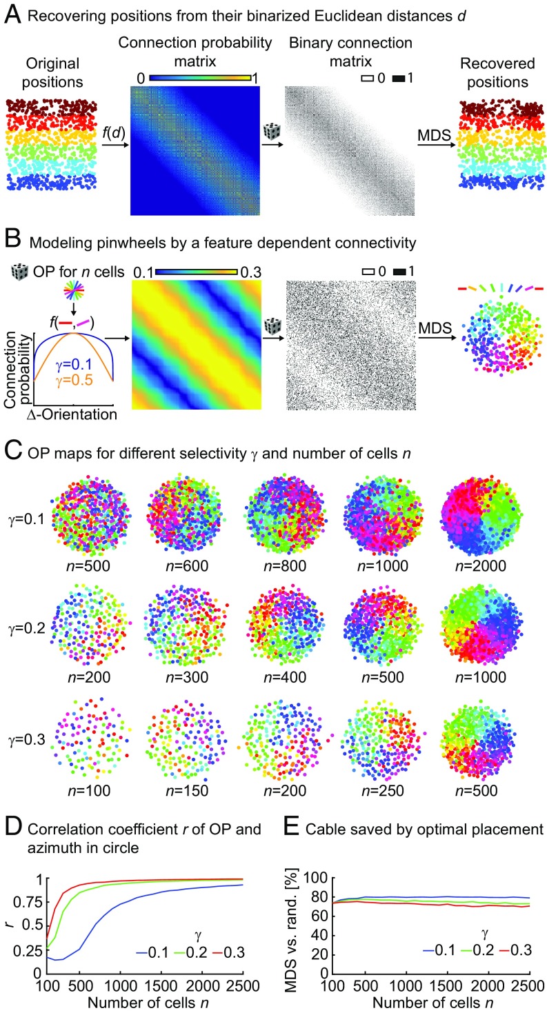
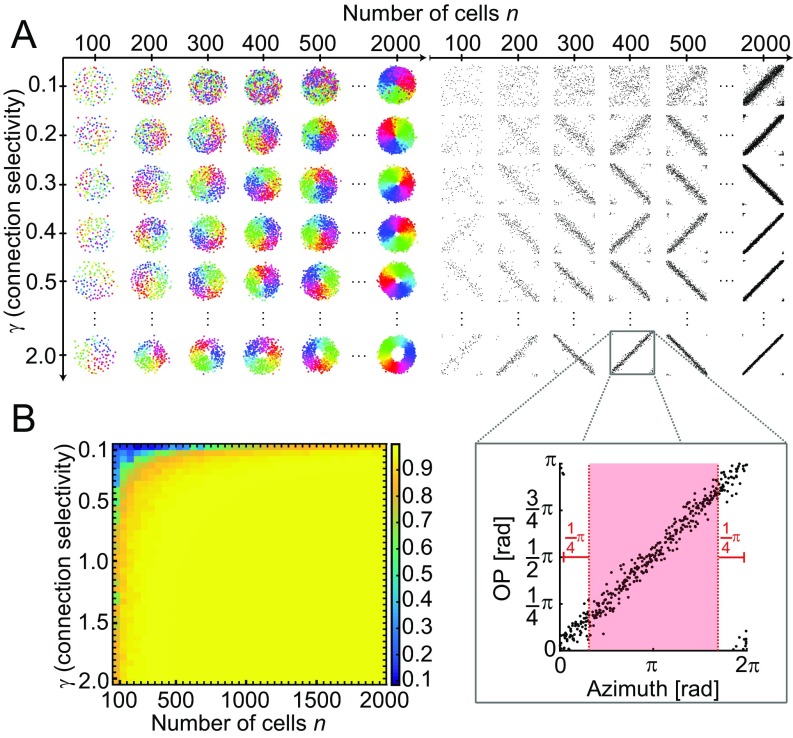
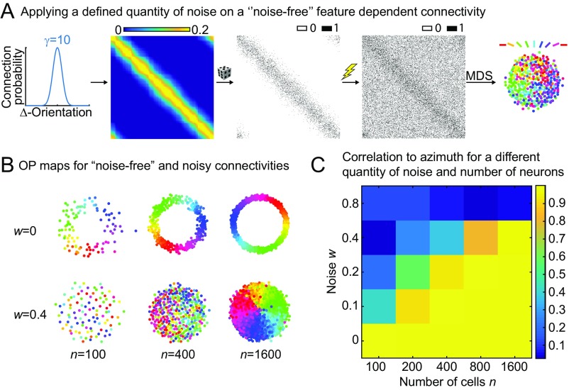
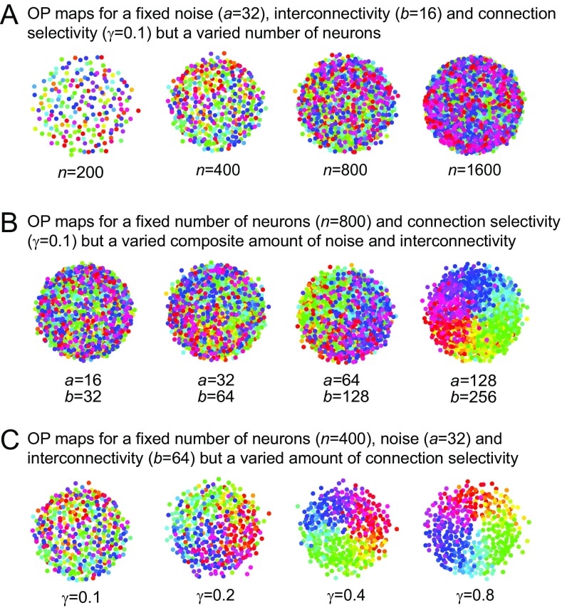
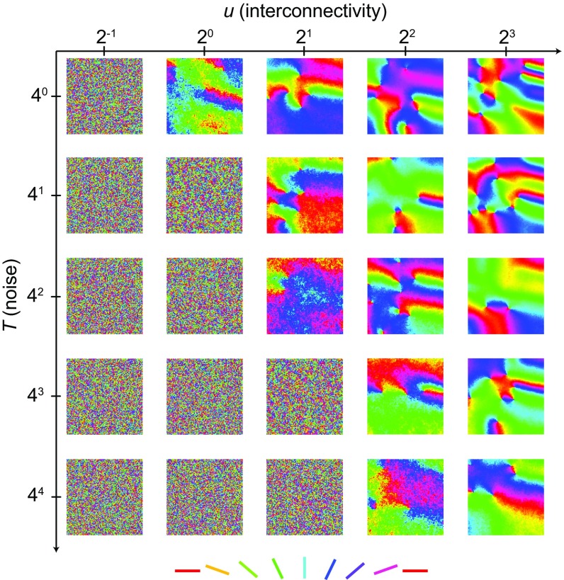
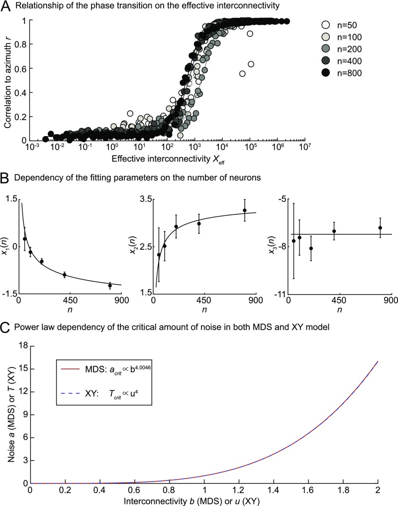
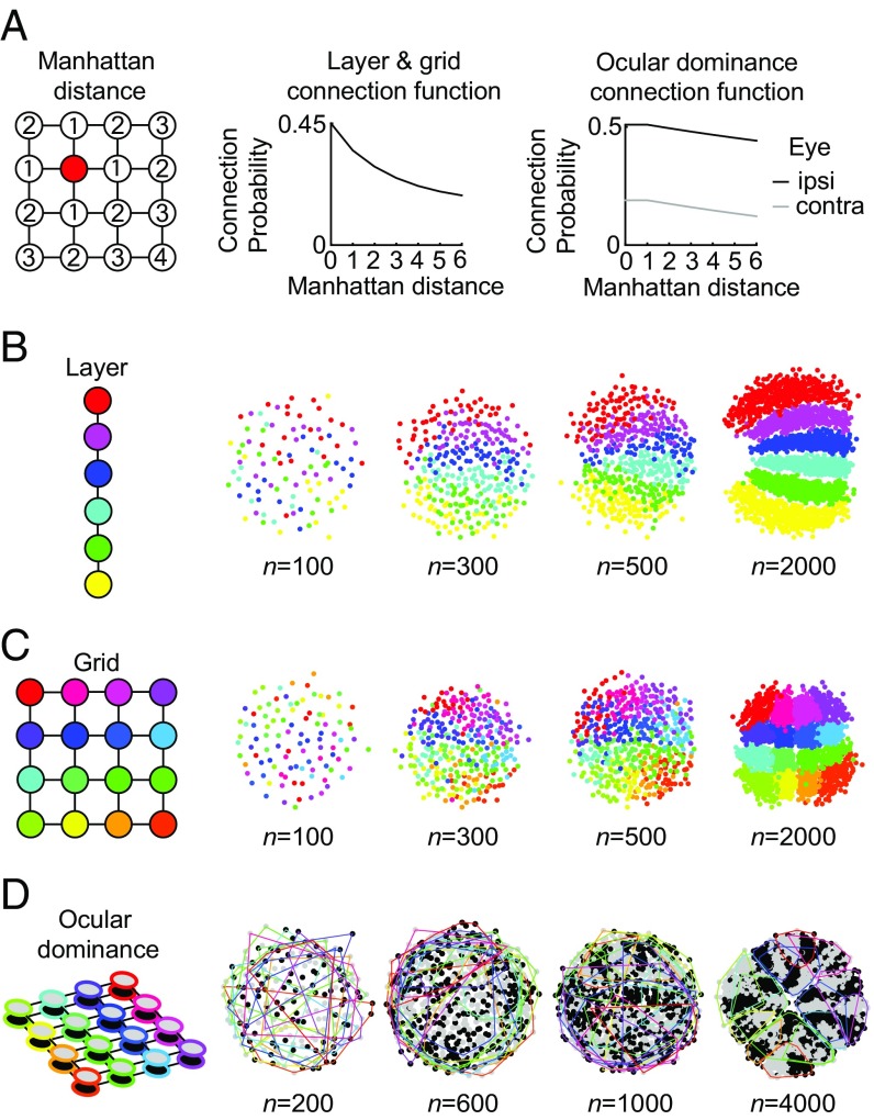
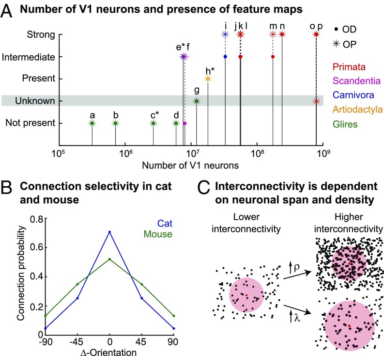
Neurons sharing similar features are often selectively connected with a higher probability and should be located in close vicinity to save wiring. Selective connectivity has, therefore, been proposed to be the cause for spatial organization in cortical maps. Interestingly, orientation preference (OP) maps in the visual cortex are found in carnivores, ungulates, and primates but are not found in rodents, indicating fundamental differences in selective connectivity that seem unexpected for closely related species. Here, we investigate this finding by using multidimensional scaling to predict the locations of neurons based on minimizing wiring costs for any given connectivity. Our model shows a transition from an unstructured salt-and-pepper organization to a pinwheel arrangement when increasing the number of neurons, even without changing the selectivity of the connections. Increasing neuronal numbers also leads to the emergence of layers, retinotopy, or ocular dominance columns for the selective connectivity corresponding to each arrangement. We further show that neuron numbers impact overall interconnectivity as the primary reason for the appearance of neural maps, which we link to a known phase transition in an Ising-like model from statistical mechanics. Finally, we curated biological data from the literature to show that neural maps appear as the number of neurons in visual cortex increases over a wide range of mammalian species. Our results provide a simple explanation for the existence of salt-and-pepper arrangements in rodents and pinwheel arrangements in the visual cortex of primates, carnivores, and ungulates without assuming differences in the general visual cortex architecture and connectivity.

Keywords: neural maps; optimal wiring; orientation preference; pinwheels; visual cortex.

Fig. 1.

Optimal placement of orientation-selective neurons switches from salt and pepper to pinwheel. (A) Validation of optimal placement using MDS (Methods). From left to right, random locations in a unit square divided into six layers by color, connection probabilities obtained from Euclidean distances [f(d)], binary connection matrix obtained by random instantiation from the connection probability matrix, and recovered positions of neurons using MDS to minimize the amount of cable for the binary connectivity matrix. Colors correspond to layers in the original locations. (B) Optimal placement for orientation-selective neurons. From left to right, connection probability obtained as a periodic function of the difference between randomly selected OPs between n neurons illustrated here for different values of γ, the selectivity of the connection (constants a and b are set to 0.1 and 0.2, respectively); connection probability matrix for γ = 0.6 and 300 neurons with uniformly distributed random OPs; randomly instantiated binary connectivity from connection probability matrix; and positions of neurons as determined using MDS. (C) Transition between salt and pepper and pinwheels. Optimal placement for different numbers of neurons n and different selectivity values γ. (D) Absolute values of correlation coefficients r between OP and azimuth for three values of γ from C using the mean of 40 instantiations of connectivity matrices (in steps of 100 cells) for each parameter combination. (E) Amount of cable used after optimal placement using MDS compared with random (rand) placement (same data as D).

Fig. S1.

Optimal placement of orientation-selective neurons for a wide range of connection selectivity values γ and numbers of neurons n. (A) Transition between salt and pepper and pinwheels. (Left) Optimal placement for different numbers of neurons n and different connection selectivity values γ. (Right) Plots with OP and azimuth for each neuron (black dots; one representative case is shown in Inset) in all combinations of γ and n from Left. (B) Absolute values of correlation coefficients between OP and azimuth for the parameter space from A but using the mean of five different instantiations of each parameter combination. Bins are 50 wide and 0.05 tall, with blue being salt and pepper (no correlation) and yellow being pinwheel (strong correlation). All correlation coefficients were calculated for the red area in B, Right to avoid the edge effects caused by the periodicity of the data. The constants a and b were set to 0.1 and 0.2, respectively, for all of the shown calculations.

Fig. S2.

Influence of noise on the optimal placement of orientation-selective neurons. (A) A highly selective noise-free connection function is used (γ = 10) to generate a connection matrix that accordingly is also noise-free. Noise is then applied by randomly setting a bin in the connection matrix to either zero or one, where the probability to change a bin is given by the noise parameter w. (B) OP maps for noise-free and noisy connectivities (w = 0.4). (C) Correlation to azimuth for more extensive parameter values of n and w. The constants a and b were set to 0 and 0.2, respectively, for all of the shown calculations.

Fig. S3.

Relationship between the interconnectivity and the number of neurons in the MDS model. (A) OP maps for different numbers of neurons but fixed parameters for noise, interconnectivity, and connection selectivity. (B) OP maps for a varied composite amount of interconnectivity and noise but a fixed number of neurons and connection selectivity. (C) OP maps for a varied connection selectivity but a fixed number of neurons, noise, and interconnectivity.

Fig. 2.

Phase transitions in the XY model with network interconnectivity. Single realizations for 25 different combinations of two parameters T and u of our adaptation of the XY model after evolving the spins on a regular lattice with up to 10 million iterations using a hybrid Monte Carlo algorithm (as described in Methods). Values are given in arbitrary units.

Fig. S4.

Relationship between phase transitions in the MDS and the XY models. (A) Fit of the correlation to the azimuth r of OP maps calculated with our MDS model for different numbers of neurons (shown as different shades of gray) and a large range of values for a and b. Original data points are shown in the space of the effective interconnectivity X_eff, which was calculated using the fitted parameters. The following ranges of a and b values have been used to obtain the fits for different numbers of neurons: n = 50 (a = [1.4236, 34.1995]; b = [1.3594, 21.5443]), n = 100 (a = [1.4236, 69.3145]; b = [1.3594, 39.8107]), n = 200 (a = [1.4236, 140.4844]; b = [1.3594, 73.5642]), n = 400 (a = [1.4236, 200]; b = [1.3594, 100]), and n = 400 (a = [1.4236, 200]; b = [1.3594, 100]). (B) Dependency of the fitting parameters (Left) x₁, (Center) x₂, and (Right) x₃ on the number of neurons n. Data points show the mean values, and the error bars show the lower and upper limits of the respective fitting parameters. Lines are fits of the dependency of x₁, x₂, and x₃ on logarithmic [$x_1\left(n\right)=A+B/\log \left(N\right)$ with A = −3.56 and B = 15.96], square root [$x_2\left(n\right)=A+B/\sqrt{N}$ with A = 3.54 and B = −9.46], and constant [$x_3\left(n\right)=A$ with A = −7.22] functions. (C) Critical noise has a power law dependence on the interconnectivity in the MDS and the XY models as shown by the curves and the given relationship in Inset. The power law of the MDS model depicted here was obtained for n = 284.

Fig. 3.

Emergence of topographic maps with increasing interconnectivity. (A, Left) Distances in the topographic arrangements were defined using the Manhattan distance. (A, Center) Connection probability for the layer and grid arrangements in B and C. (A, Right) Individual connection probabilities to ipsilateral (black) and contralateral (gray) eye. (B–D) Neural placement similar to Fig. 1C as a function of numbers of cells using the connection probabilities from A. (B) 1D connectivity leading to layers. (C) 2D grid leading to a topographic map. (D) OD arrangement connecting two 4 × 4 grids. Colors of the neurons in all panels correspond to the colors in the sketch of the connectivity arrangement on the left. For D, eye preferences are plotted in black and gray, whereas assignment to the grid is shown as convex hulls around all neurons of the same groups in their respective colors. In B–D, the resulting maps were rotated and flipped manually to best match the schematic layout.

Fig. 4.

Interpretation of the parameters and biological data. (A) Numbers of neurons in visual cortex (V1) of species from different orders (color-coded) and their relation to map structure. OD and OP map structure are given by the positions of the dot and star symbol, respectively on the y axis of the plot. Number of V1 neurons and map structure were both curated from the literature and are summarized in Tables S1 and S2. The following species are shown: (a) mouse, (b) rat, (c) gray squirrel, (d) rabbit, (e) ferret, (f) tree shrew, (g) agouti, (h) sheep, (i) cat, (j) marmoset, (k) galago, (l) owl monkey, (m) squirrel monkey, (n) macaque, (o) human, and (p) chimpanzee. Neuronal numbers for species denoted with a star are only estimates (Table S1). (B) Connection selectivity given by the connection probability between orientation-selective neurons in the visual cortices of mouse and cat (estimated mean of curated data from figure 3 in ref. ; original data from refs. , , and 71). (C) The amount of interconnectivity is dependent on both the cell density ρ and the neuronal span λ when the probability of connection within λ is constant. This relationship is illustrated as an example for one neuron (red dot) that has a fixed connection probability to other neurons (black dots) within its neuronal span (red-shaded area).

References

1. Cherniak C. Component placement optimization in the brain. J Neurosci. 1994;14:2418–2427. - PMC - PubMed
1. Cherniak C, Mokhtarzada Z, Rodriguez-Esteban R, Changizi K. Global optimization of cerebral cortex layout. Proc Natl Acad Sci USA. 2004;101:1081–1086. - PMC - PubMed
1. Mitchison G. Axonal trees and cortical architecture. Trends Neurosci. 1992;15:122–126. - PubMed
1. Bullmore E, Sporns O. The economy of brain network organization. Nat Rev Neurosci. 2012;13:336–349. - PubMed
1. Chklovskii DB, Koulakov AA. Maps in the brain: What can we learn from them? Annu Rev Neurosci. 2004;27:369–392. - PubMed
Publication types
LinkOut - more resources