Widespread Allelic Heterogeneity in Complex Traits

Abstract

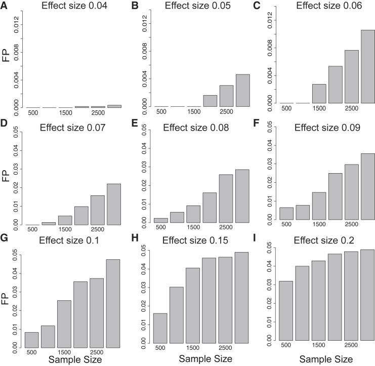
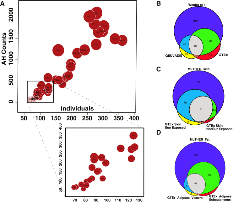
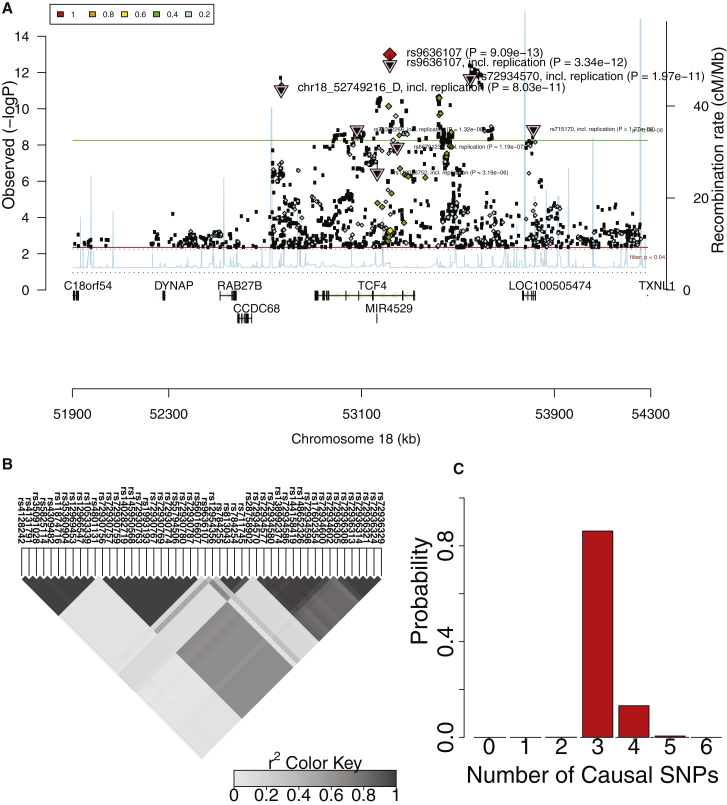
Recent successes in genome-wide association studies (GWASs) make it possible to address important questions about the genetic architecture of complex traits, such as allele frequency and effect size. One lesser-known aspect of complex traits is the extent of allelic heterogeneity (AH) arising from multiple causal variants at a locus. We developed a computational method to infer the probability of AH and applied it to three GWASs and four expression quantitative trait loci (eQTL) datasets. We identified a total of 4,152 loci with strong evidence of AH. The proportion of all loci with identified AH is 4%-23% in eQTLs, 35% in GWASs of high-density lipoprotein (HDL), and 23% in GWASs of schizophrenia. For eQTLs, we observed a strong correlation between sample size and the proportion of loci with AH (R² = 0.85, p = 2.2 × 10^-16), indicating that statistical power prevents identification of AH in other loci. Understanding the extent of AH may guide the development of new methods for fine mapping and association mapping of complex traits.

Keywords: allelic heterogeneity; causal variants; complex traits; eQTL; gene expression.

Figure 1

Overview of CAVIAR for Detecting Allelic Heterogeneity Regions (A and B) The marginal statistics for a locus where we have implanted one causal variant. In (A), SNP33 is causal and in (B), SNP23 is causal. (C) The same locus where both SNP23 and SNP33 are causal. In these figures, the x axis is the negative logarithm of the p values for each locus to indicate the strength of the marginal statistics. The gray triangle below each figure indicates the LD pattern. Each square indicates the correlation between two variants, and the magnitude of the correlation is shown by the color intensity of the square. The darker the square, the higher the correlation between two variants.

Figure 2

ROC Curve for CAVIAR and CM We implant one causal variant to compute the false positive (FP) rate. FP indicates loci that harbor one causal variant; however, these loci are detected as AH. We implant two causal variants to compute the true positive (TP) rate. TP indicates loci that harbor AH and are detected correctly. We range the effect size such that the power at the causal variant is 20%, 40%, 60%, and 80% at the genome significant level 10⁻⁸. We obtain these results from simulated data with no epistasis interaction. We simulated data using 1,000 individuals and set γ to 0.001.

Figure 3

CAVIAR Has Low FP Even When the True Causal Variant Is Not Collected Thus, most loci that are detected by CAVIAR to harbor AH are most probably true. x axis indicates the prior probability of causal variant (γ). We set γ to 0.01, 0.005, 0.001, 0.0005, 0.0001, 0.00005, 0.000001, and 0.000005.

Figure 4

CAVIAR Is More Accurate than CM to Detect the Number of Causal Variants The x axis is the power of causal variants, and the y axis is the accuracy to detect the number of causal variants in a locus. We implanted one, two, and three causal variants. We compute the recall rate as the fraction of simulations where the number of causal variants in a locus is predicted correctly. Recall rate of each method for different number of causal variants: (A) one causal variant, (B) two causal variants, and (C) three causal variants. We vary the statistical power to detect the causal variant among 0.2, 0.3, 0.4, 0.5, 0.6, 0.7, and 0.8.

Figure 5

CAVIAR Distinguishes between Epistatic Interaction and Allelic Heterogeneity The x axis is the sample size that we vary between 500, 1,000, 1,500, 2,000, 2,500, and 3,000 individuals. The y axis is the false positive (FP) rate. We simulated datasets where we have epistatic interaction and compute the FP as the number of cases where CAVIAR incorrectly detects these loci to harbor AH. Shown are the FP for different effect sizes of the epistatic interaction.

Figure 6

Levels of Allelic Heterogeneity in eQTL Studies (A) Linear relationship between the amount of AH and sample size. Each red circle indicates a different type of tissue from the GTEx dataset. The size of each red circle is proportional to the number of genes that harbor a significant eQTL (eGenes). (B–D) Significant overlap between AH estimations for different eQTL datasets, shown for (B) blood (p = 7.9 × 10⁻⁹⁷), (C) skin (p = 4.9 × 10⁻⁶³), and (D) adipose (p = 1.1 × 10⁻⁶⁹) tissue. p values are computed using a hypergeometric test that is implemented in the SuperExactTest software.

Figure 7

Allelic Heterogeneity in the TCF4 Locus Associated with Schizophrenia (A) Manhattan plot obtained from Ricopili consists of all the variants (7,193 variants) in a 1 Mbp window centered on the most significant SNP in the locus (rs9636107). We use PGC-SCZ52-may13 version of the data. This plot indicates multiple significant variants that are not in tight LD with the peak variant. (B) LD plot of the 50 most significant SNPs showing several distinct LD blocks. (C) Histogram for the probability of having different number of causal variants.

References

1. Wellcome Trust Case Control Consortium Genome-wide association study of 14,000 cases of seven common diseases and 3,000 shared controls. Nature. 2007;447:661–678. - PMC - PubMed
1. Rietveld C.A., Medland S.E., Derringer J., Yang J., Esko T., Martin N.W., Westra H.-J., Shakhbazov K., Abdellaoui A., Agrawal A., LifeLines Cohort Study GWAS of 126,559 individuals identifies genetic variants associated with educational attainment. Science. 2013;340:1467–1471. - PMC - PubMed
1. Ripke S., Neale B.M., Corvin A., Walters J.T.R., Farh K.-H., Holmans P.A., Lee P., Bulik-Sullivan B., Collier D.A., Huang H., Schizophrenia Working Group of the Psychiatric Genomics Consortium Biological insights from 108 schizophrenia-associated genetic loci. Nature. 2014;511:421–427. - PMC - PubMed
1. Barrett J.C., Clayton D.G., Concannon P., Akolkar B., Cooper J.D., Erlich H.A., Julier C., Morahan G., Nerup J., Nierras C., Type 1 Diabetes Genetics Consortium Genome-wide association study and meta-analysis find that over 40 loci affect risk of type 1 diabetes. Nat. Genet. 2009;41:703–707. - PMC - PubMed
1. Zhang F., Lupski J.R. Non-coding genetic variants in human disease. Hum. Mol. Genet. 2015;24(R1):R102–R110. - PMC - PubMed