Breast MRI segmentation for density estimation: Do different methods give the same results and how much do differences matter?

Abstract

Purpose: To compare two methods of automatic breast segmentation with each other and with manual segmentation in a large subject cohort. To discuss the factors involved in selecting the most appropriate algorithm for automatic segmentation and, in particular, to investigate the appropriateness of overlap measures (e.g., Dice and Jaccard coefficients) as the primary determinant in algorithm selection.

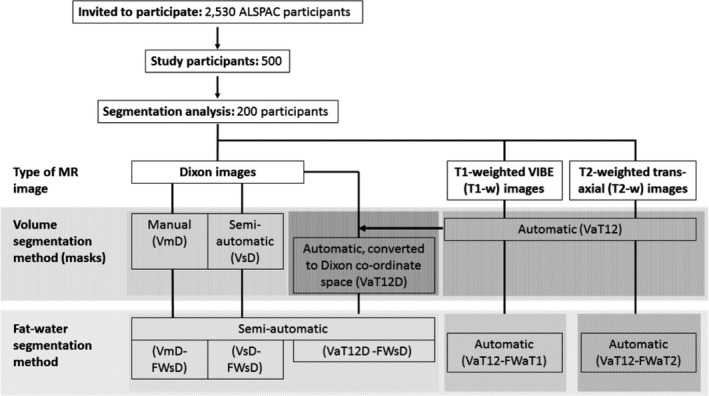
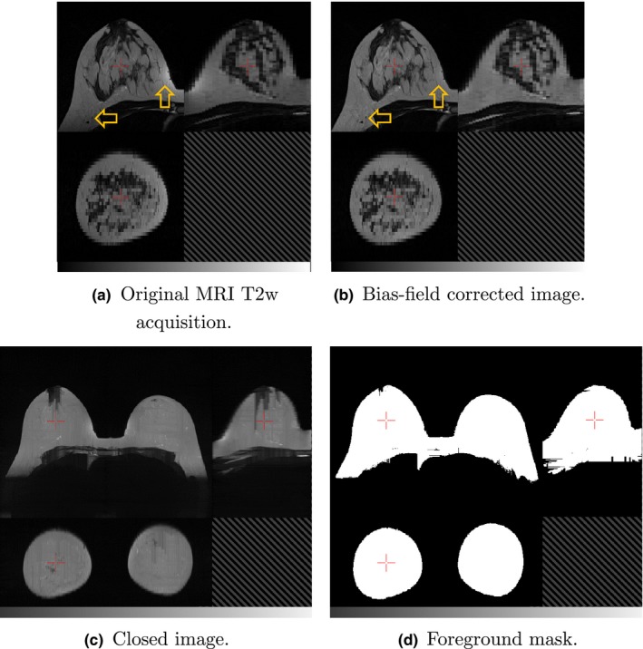
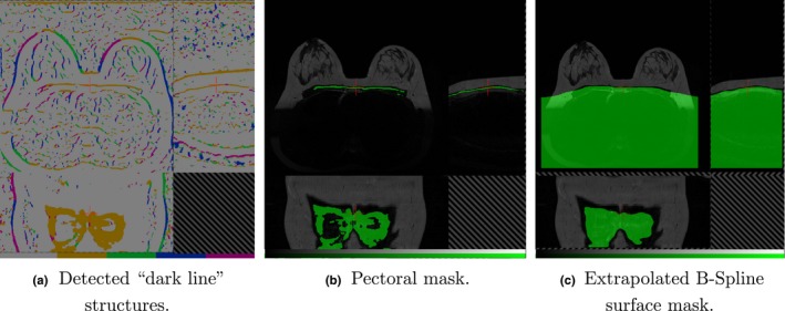
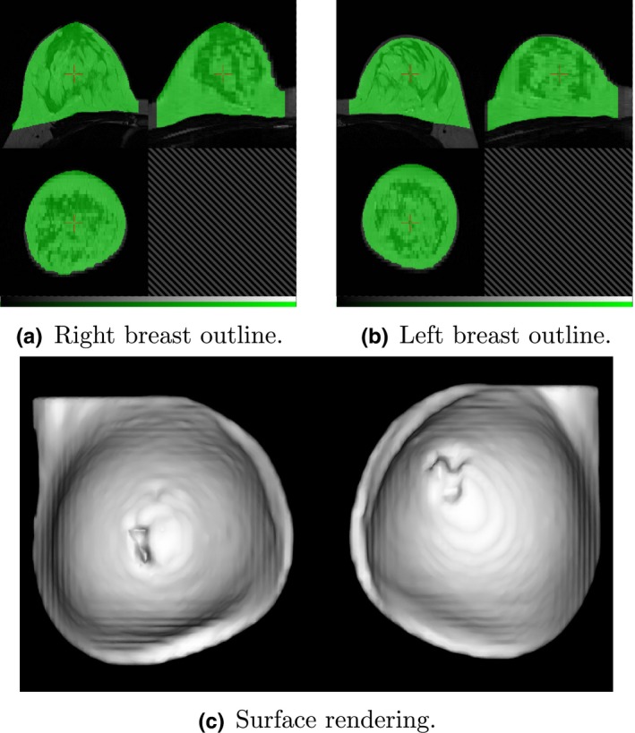
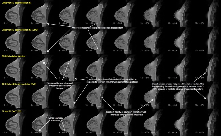
Methods: Two methods of breast segmentation were applied to the task of calculating MRI breast density in 200 subjects drawn from the Avon Longitudinal Study of Parents and Children, a large cohort study with an MRI component. A semiautomated, bias-corrected, fuzzy C-means (BC-FCM) method was combined with morphological operations to segment the overall breast volume from in-phase Dixon images. The method makes use of novel, problem-specific insights. The resulting segmentation mask was then applied to the corresponding Dixon water and fat images, which were combined to give Dixon MRI density values. Contemporaneously acquired T₁ - and T₂ -weighted image datasets were analyzed using a novel and fully automated algorithm involving image filtering, landmark identification, and explicit location of the pectoral muscle boundary. Within the region found, fat-water discrimination was performed using an Expectation Maximization-Markov Random Field technique, yielding a second independent estimate of MRI density.

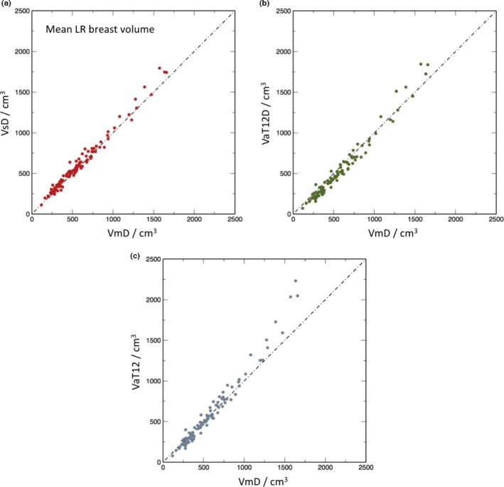
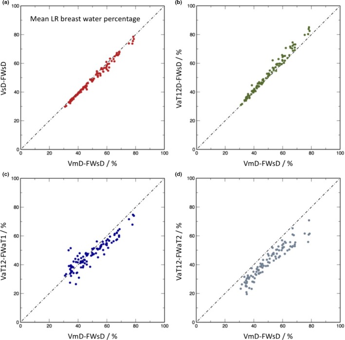
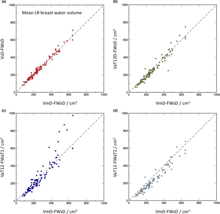
Results: Images are presented for two individual women, demonstrating how the difficulty of the problem is highly subject-specific. Dice and Jaccard coefficients comparing the semiautomated BC-FCM method, operating on Dixon source data, with expert manual segmentation are presented. The corresponding results for the method based on T₁ - and T₂ -weighted data are slightly lower in the individual cases shown, but scatter plots and interclass correlations for the cohort as a whole show that both methods do an excellent job in segmenting and classifying breast tissue.

Conclusions: Epidemiological results demonstrate that both methods of automated segmentation are suitable for the chosen application and that it is important to consider a range of factors when choosing a segmentation algorithm, rather than focus narrowly on a single metric such as the Dice coefficient.

Keywords: ALSPAC; MRI; breast cancer; mammographic density; segmentation.

Figure 1

Flow diagram of the overall data processing chain and nomenclature for the various segmentation methods. Some of these have the potential to operate on different source data and we can also combine the methods in different ways to achieve an overall result. We thus assign each step three codes: segmentation purpose (V = breast volume, FW = fat–water); degree of automation (m = manual, s = semi‐automatic, a = fully automatic); and source data (D = Dixon; T1 = T ₁‐weighted, T2 = T ₂‐weighted, T12 = uses both T ₁‐ and T ₂‐weighted data). Thus, a breast‐volume measurement using semiautomatic segmentation on original Dixon data would be represented as VsD. Fat–water segmentations require both source data and a previously generated volume mask, so are represented by the combination of two codes. For instance, fat–water statistics calculated semiautomatically from Dixon source data and using a mask generated automatically from T1w and T2w data would be described by VaT12‐FWsD. We note one additional case, in which the volume mask VaT12 is re‐sampled to give a result in the same coordinate space as the Dixon images and we assign this the label VaT12D.

Figure 2

Orthogonal slices through (a) a T2 weighted MRI and (b) the corresponding image after bias‐field correction, with arrows indicating regions that are particularly improved by the processing. The “closed” T2w image is shown in (c) and foreground mask I _fg in (d). In each image, the top‐left quadrant is the axial slice, the top‐right is sagittal and the bottom‐left is coronal. [Color figure can be viewed at wileyonlinelibrary.com]

Figure 3

The anterior pectoral muscle surface is detected using the Oriented Basic Image Feature “dark line” class. Subplot (a) shows these features detected at four orientations (OBIF₁₅ to OBIF₁₈). Region growing the “brown” medial‐lateral class, OBIF₁₅, closely delineates this anterior boundary immediately posterior to the sternum (b). The anterior surface of this mask is extrapolated using a B‐Spline fit to the lateral boundaries of the volume (c). [Color figure can be viewed at wileyonlinelibrary.com]

Figure 4

Breast region mask created by removing the pectoral surface mask (Fig. 3) from the foreground mask (Fig. 2). Two views of the mask are shown, superimposed on the original MR image and centered on the right (a) and left (b) breasts. The surface rendering (c) illustrates the “squaring off” to include the axilla. [Color figure can be viewed at wileyonlinelibrary.com]

Figure 5

Example of a case where both of the algorithms examined in this work performed well. Features of interest in the various different segmentations are annotated. Note that this image is provided with high resolution and can be zoomed significantly to reveal additional detail. [Color figure can be viewed at wileyonlinelibrary.com]

Figure 6

Example of a case where automatic segmentation is difficult. The rows represent the results of different segmentations and, for compactness, an informative subset of slices has been chosen to illustrate important features of the problem. Note that this image is provided with high resolution and can be zoomed significantly to reveal additional detail. [Color figure can be viewed at wileyonlinelibrary.com]

Figure 7

Scatter plots of mean left and right breast volumes in cm³ for the different methods in comparison to manual segmentation: (a) volume from semiautomatic segmentation of Dixon images (VsD) vs. volume from manual segmentation (VmD); (b) volume via automated segmentation from T₁‐ and T₂‐weighted images transformed to Dixon reference frame (VaT12FD) vs manual (VmD); (c) volume obtained from T₁‐ and T₂‐weighted images in native 3‐D reference frame (VaT12). [Color figure can be viewed at wileyonlinelibrary.com]

Figure 8

Scatter plots of mean left and right breast water percentage for the different methods in comparison with manual segmentation on Dixon images followed by percentage water estimation the using semiautomated Dixon image method: (a) semiautomatic segmentation of Dixon images followed by percentage estimate from Dixon image data (VsD‐FWsd); (b) volume via automated segmentation from T₁‐ and T₂‐weighted images transformed to Dixon reference frame (VaT12FD) followed by semiautomated percentage estimate from the Dixon data (VaT12D‐FWsd); (c) volume obtained from T₁‐ and T₂‐weighted images in native 3‐D reference frame, followed by automatic percentage estimate from T₁‐weighted data (VaT12‐FWaT1); (d) as (c), but with the water percentage estimated from the T₂‐weighted data. [Color figure can be viewed at wileyonlinelibrary.com]

Figure 9

Scatter plots of mean left and right breast water volumes in cm³ for the different methods in comparison to VmD‐FWsD. For nomenclature see caption to Fig. 8. [Color figure can be viewed at wileyonlinelibrary.com]

Figure 10

Results of epidemiological analysis. Relative change in geometric means of MR breast volume and percent water in relation to a unit increase, or category change, in each breast composition correlate variable. ¹Models adjusted for current age in months and BMI at MR scan, where appropriate. ²Models restricted to young women for whom mammograms from their mothers could be retrieved (n = 33) adjusted for current age in months and BMI at MR scan and maternal age at mammogram and BMI in 2010 (median = 3y (IQR = 1.5y) prior to mammogram). For further details, see Supplementary Information. [Color figure can be viewed at wileyonlinelibrary.com]

References

1. McCormack VA, Silva IDS. Breast density and parenchymal patterns as markers of breast cancer risk: a meta‐analysis. Cancer Epidemiol Biomarkers Prev. 2006;15:1159–1169. - PubMed
1. Vilaprinyo E, Forne C, Carles M, et al. Cost‐effectiveness and harm‐benefit analyses of risk‐based screening strategies for breast cancer. Plos One. 2014;9:e86858. - PMC - PubMed
1. Price ER, Keedy AW, Gidwaney R, Sickles EA, Joe BN. The potential impact of risk‐based screening mammography in women 40‐49 years old. Am J Roentgenol. 2015;205:1360–1364. - PubMed
1. Ciatto S, Houssami N, Apruzzese A, et al. Categorizing breast mammographic density: intra‐ and interobserver reproducibility of bi‐rads density categories. Breast 2005;14:269–275. - PubMed
1. Highnam R, Brady SM, Yaffe MJ, Karssemeijer N, Harvey J. Robust breast composition measurement ‐ volparatm In: Mart J, Oliver A, Freixenet J, Mart R, eds. Digital Mammography: 10th International Workshop, IWDM 2010, Girona, Catalonia, Spain, June 16–18, 2010. Proceedings. Berlin, Heidelberg: Springer Berlin Heidelberg; 2010: 342–349.