An Evaluation of the Accuracy of Classical Models for Computing the Membrane Potential and Extracellular Potential for Neurons

Abstract

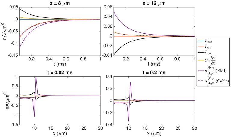
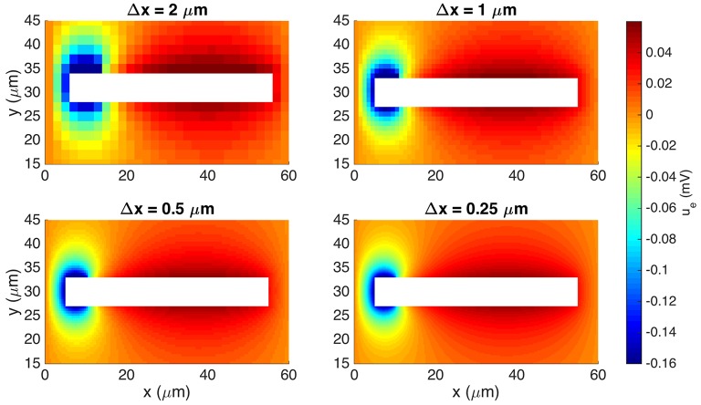
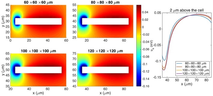
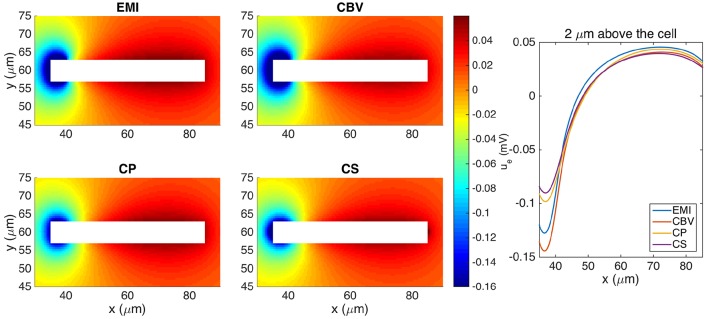
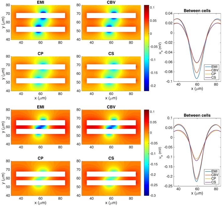
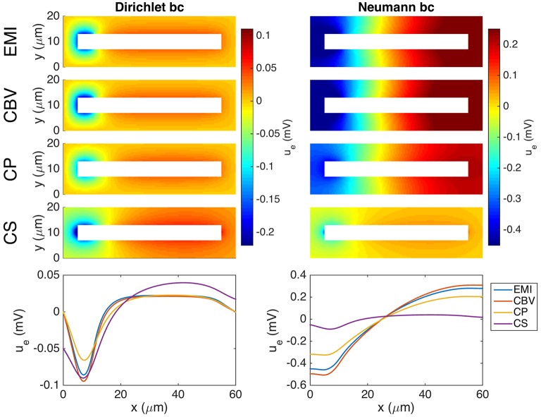
Two mathematical models are part of the foundation of Computational neurophysiology; (a) the Cable equation is used to compute the membrane potential of neurons, and, (b) volume-conductor theory describes the extracellular potential around neurons. In the standard procedure for computing extracellular potentials, the transmembrane currents are computed by means of (a) and the extracellular potentials are computed using an explicit sum over analytical point-current source solutions as prescribed by volume conductor theory. Both models are extremely useful as they allow huge simplifications of the computational efforts involved in computing extracellular potentials. However, there are more accurate, though computationally very expensive, models available where the potentials inside and outside the neurons are computed simultaneously in a self-consistent scheme. In the present work we explore the accuracy of the classical models (a) and (b) by comparing them to these more accurate schemes. The main assumption of (a) is that the ephaptic current can be ignored in the derivation of the Cable equation. We find, however, for our examples with stylized neurons, that the ephaptic current is comparable in magnitude to other currents involved in the computations, suggesting that it may be significant-at least in parts of the simulation. The magnitude of the error introduced in the membrane potential is several millivolts, and this error also translates into errors in the predicted extracellular potentials. While the error becomes negligible if we assume the extracellular conductivity to be very large, this assumption is, unfortunately, not easy to justify a priori for all situations of interest.

Keywords: cable equation; ephaptic coupling; extracellular potential; membrane potentials; numerical modeling.

Figure 1

Sketch of a simplified neuron of rectangular cuboid shape with dimensions l_x, l_y, and l_z. The intracellular domain is denoted Ω_i, the boundary is Γ, and the compartments of length Δx are denoted by Ω_{i, k}.

Figure 2

Sketch of a simplified neuron geometry and its surroundings; the extracellular domain Ω_e, the cell membrane Γ, and the intracellular domain Ω_i. The normal vector pointing out of Ω_i, is denoted by n_i and, similarly, n_e denotes the normal vector pointing out of Ω_e.

Figure 3

Sketch of the computational mesh for Ω_e and Ω_i; the nodes of Ω_e are marked by “×,” the nodes of Ω_i are marked by “°,” and the membrane is defined as the intersection of Ω_e and Ω_i marked by “⊗.”

Figure 4

Comparison of the membrane potential computed by solving the Cable equation (red) and the EMI model (blue) for some different values of h, σ_i, σ_e, and g_L, where we recall that h = l_y = l_z (the width of the neuron). The plots show how the membrane potential in the compartment 25 μm from the start of the cell changes with time from t = 0.1 to 0.5 ms. The parameters used in the computations are given in Table 2 except for the values given above each plot. We observe that the difference between the two solutions increases when the value of h or σ_i is increased, and the difference decreases when the value of σ_e or g_L is increased. Note that in order to observe any effect of changing the value of g_L, we increase the default value by a factor of order 100–1,000 in the lower panel of the figure.

Figure 5

Values of each of the terms in Equation (9). In the (Upper panel), we show the time evolution of the terms in the point (8, 10, 7 μm) inside the synaptic input zone and the point (12, 10, 7 μm) outside the synaptic input zone. In the (Lower panel), we show the values of the terms for y = 10 μm, z = 7 μm, and x ∈ [5 μ m, 30μm] at time t = 0.02 ms (left) and t = 0.2 ms (right). The solution of the EMI model is used to compute each of the terms. In addition, we show $\eta \frac{{\partial }^{2}v}{\partial x^2}$ for the corresponding solution of the Cable equation, where I_eph is assumed to be zero. We observe that the size of I_eph is comparable to the size of the other terms in Equation (9) and that neglecting I_eph leads to a considerable difference in the value of the term $\eta \frac{{\partial }^{2}v}{\partial x^2}$. The parameters used in the computations are given in Table 2.

Figure 6

Extracellular potential computed by the stationary EMI model for four different values of Δx = Δy = Δz. We show the solution in a rectangle of size 60 × 30 μm on the plane in the center of the domain in the z-direction. The white area represents the cell. We use the parameters given in Table 2 except for an increased value of $g_L=3·10^{-5}$ μS/μm² and a domain of size 60 × 60 × 60 μm.

Figure 7

Comparison of the extracellular potential around a neuron computed by the stationary EMI model for four different sizes of the extracellular domain. The plots to the left show the solution in a rectangle of size 60 × 30 μm on the plane in the center of the domain in the z-direction. The white area represents the neuron. The plot to the right shows the extracellular potential along a line 2 μm above the neuron in the y-direction and in the center of the domain in the z-direction. The parameters used in the computations are given in Table 2 except for L_x, L_y, and L_z, which are specified for each simulation, and g_L, which is set to 3 · 10⁻⁵ μS/μm².

Figure 8

The extracellular potential around a neuron shaped as a rectangular cuboid computed by the stationary versions of the EMI, CBV, CP, and CS methods. The plots to the left show the solution in a rectangle of size 60 × 30 μm on the plane in the center of the domain in the z-direction. The white area represents the neuron. The plot to the right shows the extracellular potential along a line 2 μm above the neuron in the y-direction and in the center of the domain in the z-direction. We use the parameters specified in Table 2 except for L_x = L_y = L_z = 120 μm and $g_L=3·10^{-5}$ μS/μm². The abbreviations (EMI, CBV, CP, and CS) are summarized in Table 1.

Figure 9

The extracellular potential around two neurons computed by the stationary versions of the EMI, CBV, CP, and CS methods. The plots to the left show the solution in a rectangle of size 60 × 40 μm on the plane in the center of the domain in the z-direction. The white areas represent the neurons. The plots to the right show the extracellular potential along the line in the center of the space between the two neurons. In the upper five plots, the neurons are separated by a distance of 10 μm in the y-direction, and in the lower five plots the neurons are separated by a distance of 4 μm. In all plots g_s(x) is given by g_syn for x ∈ [55, 60 μm] and is zero on the rest of the membrane for the lower neuron. For the upper neuron g_s(x) is given by g_syn for x ∈ [60 μm, 65 μm]. We use the parameters specified in Table 2 except for L_x = L_y = L_z = 120 μm and $g_L=3·10^{-5}$ μS/μm². The abbreviations (EMI, CBV, CP, and CS) are summarized in Table 1.

Figure 10

Extracellular potential around a neuron computed by the EMI, CBV, CP, and CS methods. We consider the stationary version of the models and the parameter values given in Table 2 except for an increased value of $g_L=3·10^{-5}\mu$m. A Dirichlet boundary condition, u_e = 0, is applied in the simulation in the left panel and a Neumann boundary condition, $\frac{\partial u_{\mathrm{\text{e}}}}{\partial n_{\mathrm{\text{e}}}}=0$, is applied in the right panel. The (Upper panels) show the extracellular potential in the plane in the center of the domain in the z-direction for each of the methods. The (Lower panel) shows the solution along a line 2 μm above the cell in the y-direction and in the center of the domain in the z-direction. Note that in the case of Neumann boundary conditions, we include the additional constraint ${\int }_{{\Omega }_{\mathrm{\text{e}}}}{u}_{\mathrm{\text{e}}}dV=0$ for the EMI, CBV, and CP methods in order to obtain unique solutions. The abbreviations (EMI, CBV, CP, and CS) are summarized in Table 1.

Figure 11

Extracellular potential around a neuron with a synaptic input area of length 5, 10, 20, and 30% of the total cell length. The (Upper panel) shows the extracellular potential computed by the EMI method in the plane in the center of the domain in the z-direction. The (Lower panel) shows the solution for each of the methods along a line 2 μm above the cell in the y-direction and in the center of the domain in the z-direction. The figure shows the solution of the stationary version of the models using the parameter values given in Table 2 except for an increased value of $g_L=3·10^{-5}\mu$m. We apply a homogeneous Dirichlet boundary condition on the outer boundary of the extracellular domain. The abbreviations (EMI, CBV, CP, and CS) are summarized in Table 1.

References

1. Agudelo-Toro A. (2012). Numerical Simulations on the Biophysical Foundations of the Neuronal Extracellular Space. Ph.D. thesis, Niedersächsische Staats-und Universitätsbibliothek Göttingen.
1. Agudelo-Toro A., Neef A. (2013). Computationally efficient simulation of electrical activity at cell membranes interacting with self-generated and externally imposed electric fields. J. Neural Eng. 10:026019. 10.1088/1741-2560/10/2/026019 - DOI - PubMed
1. Anastassiou C. A., Koch C. (2015). Ephaptic coupling to endogenous electric field activity: why bother? Curr. Opin. Neurobiol. 31, 95–103. 10.1016/j.conb.2014.09.002 - DOI - PubMed
1. Anastassiou C. A., Perin R., Markram H., Koch C. (2011). Ephaptic coupling of cortical neurons. Nat. Neurosci. 14, 217–223. 10.1038/nn.2727 - DOI - PubMed
1. Arvanitaki A. (1942). Effects evoked in an axon by the activity of a contiguous one. J. Neurophysiol. 5, 89–108.
LinkOut - more resources