Whole-brain serial-section electron microscopy in larval zebrafish

Abstract

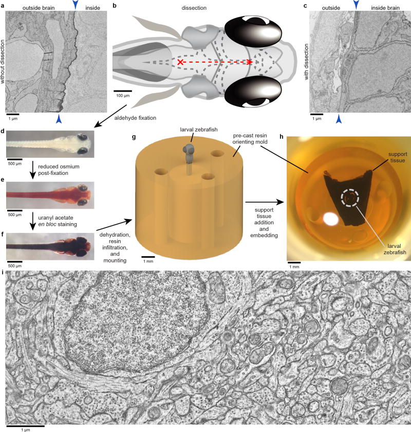
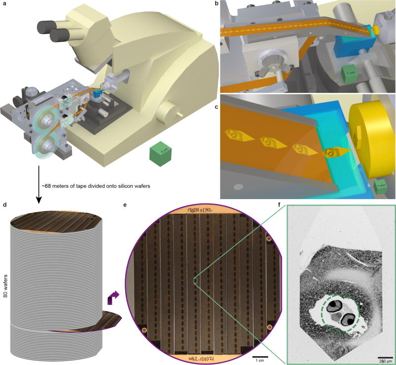
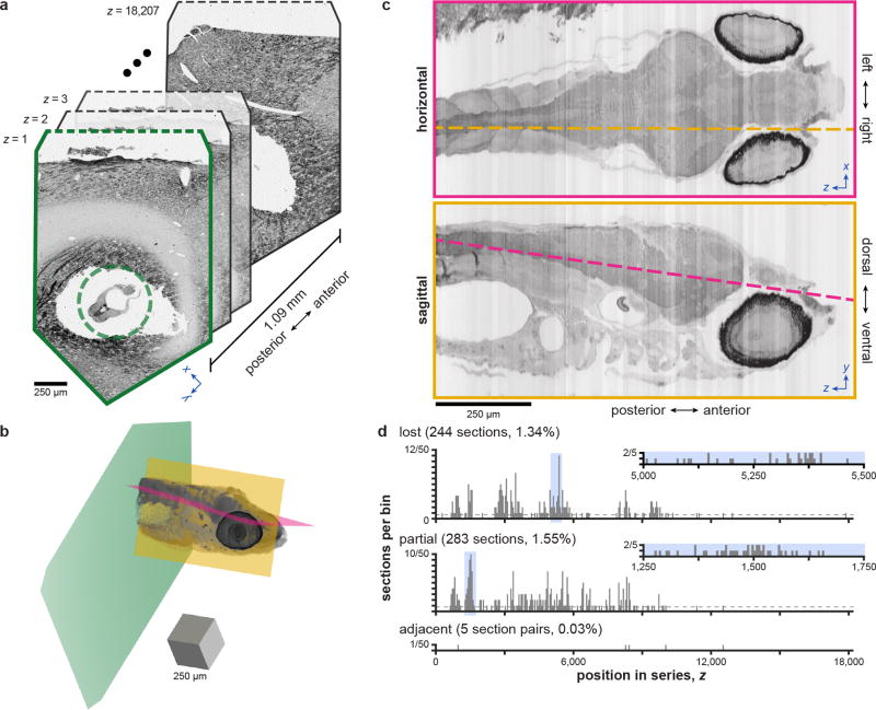
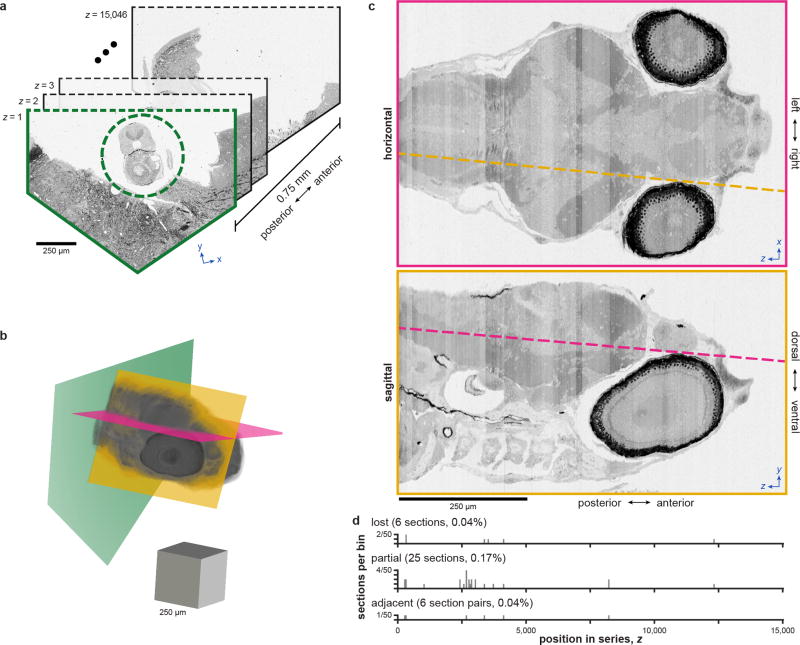
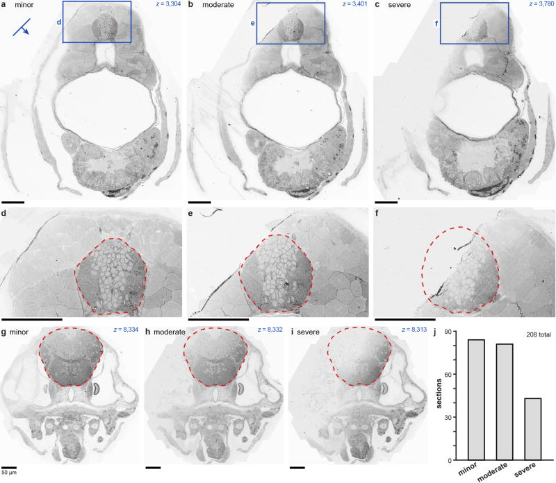
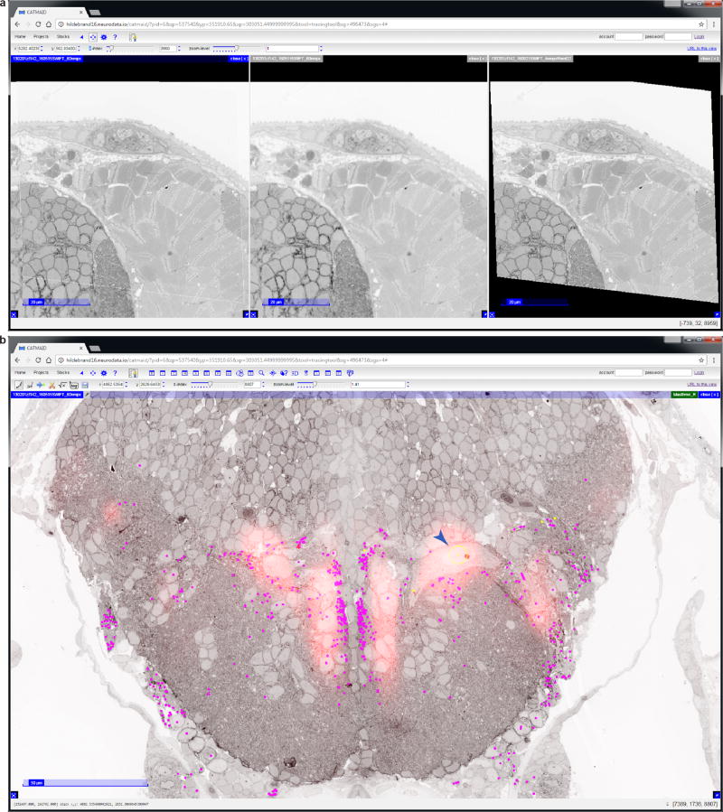
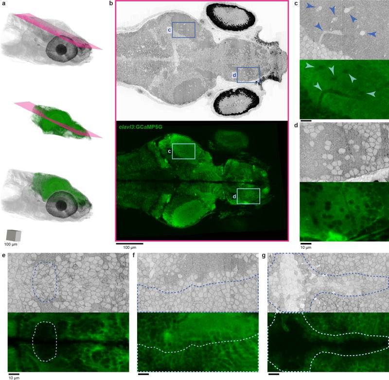
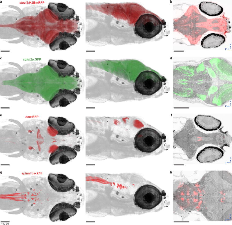
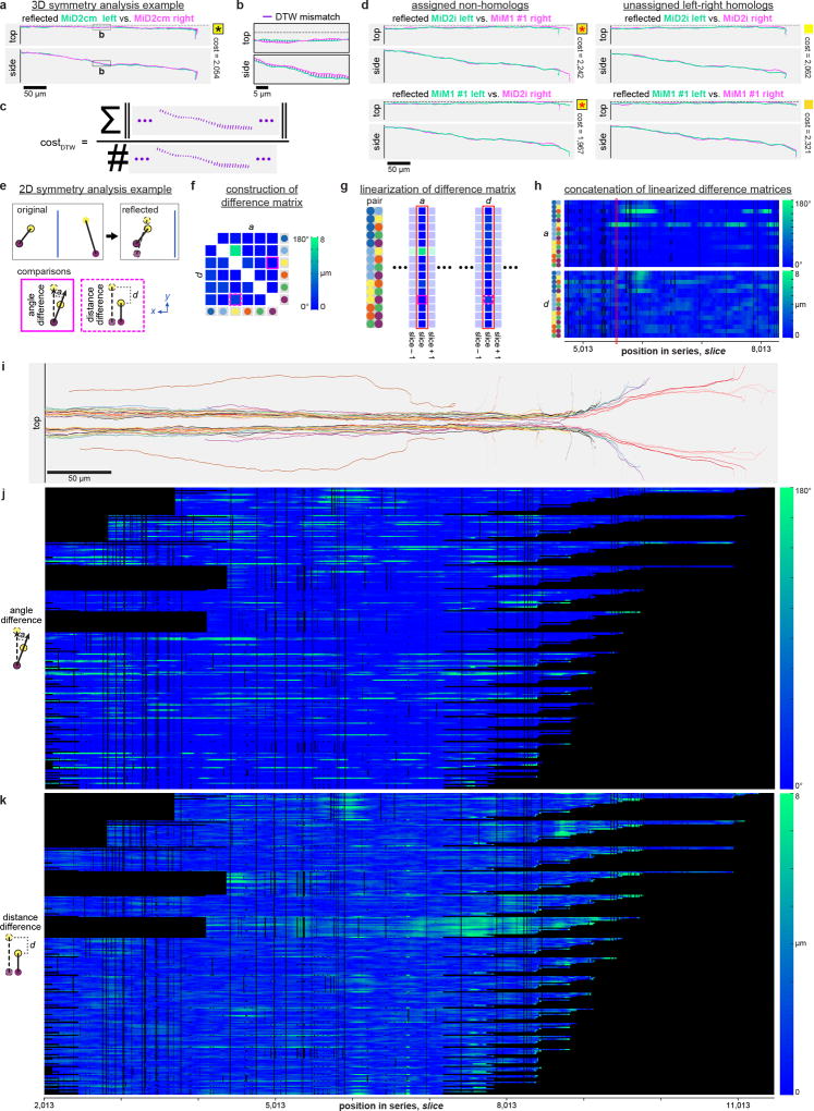
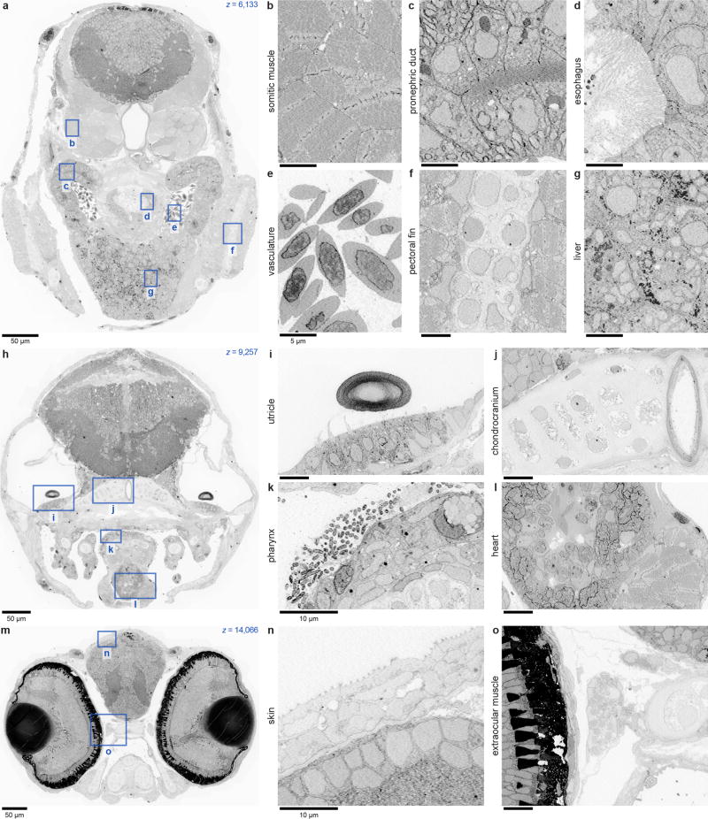
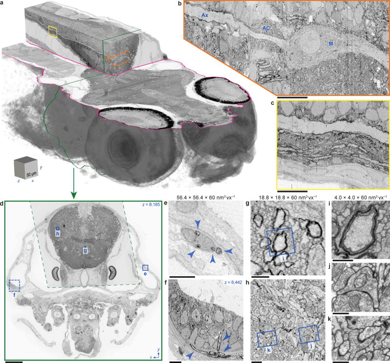
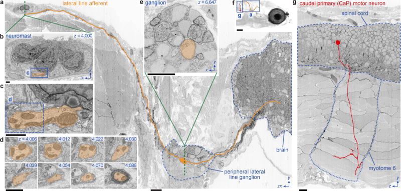
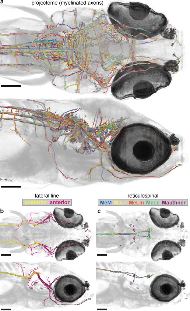
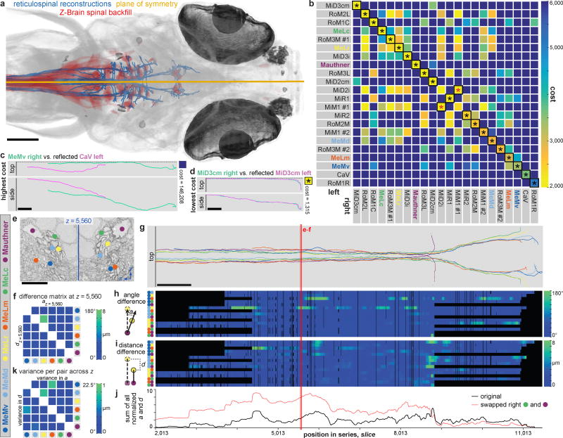
High-resolution serial-section electron microscopy (ssEM) makes it possible to investigate the dense meshwork of axons, dendrites, and synapses that form neuronal circuits. However, the imaging scale required to comprehensively reconstruct these structures is more than ten orders of magnitude smaller than the spatial extents occupied by networks of interconnected neurons, some of which span nearly the entire brain. Difficulties in generating and handling data for large volumes at nanoscale resolution have thus restricted vertebrate studies to fragments of circuits. These efforts were recently transformed by advances in computing, sample handling, and imaging techniques, but high-resolution examination of entire brains remains a challenge. Here, we present ssEM data for the complete brain of a larval zebrafish (Danio rerio) at 5.5 days post-fertilization. Our approach utilizes multiple rounds of targeted imaging at different scales to reduce acquisition time and data management requirements. The resulting dataset can be analysed to reconstruct neuronal processes, permitting us to survey all myelinated axons (the projectome). These reconstructions enable precise investigations of neuronal morphology, which reveal remarkable bilateral symmetry in myelinated reticulospinal and lateral line afferent axons. We further set the stage for whole-brain structure-function comparisons by co-registering functional reference atlases and in vivo two-photon fluorescence microscopy data from the same specimen. All obtained images and reconstructions are provided as an open-access resource.

Extended Data Figure 1. Preparing larval zebrafish brain tissue for ssEM

a, Immersion of intact specimens into tissue processing solutions resulted in poor preservation of brain ultrastructure due to membranes (arrowheads). b–c, Dissecting away the skin and membranes allowed solutions to diffuse into the brain, resulting in improved preservation. To minimize damage, dissections were initiated by puncturing the rhombencephalic ventricle dorsal to the hindbrain with a sharpened tungsten needle (red cross). Small anterior-directed incisions along the midline were then made as close to the surface as possible until the brain up to the anterior optic tectum was exposed (red dashed line). d–f, Following dissection and aldehyde fixation (d), samples were post-fixed with a reduced osmium solution (e) and stained with uranyl acetate (f). g–h, Processed specimens were then dehydrated with acetonitrile, infiltrated with a low-viscosity resin, mounted in a micromachined pre-cast resin mould to orient the sample for transverse sectioning (g), and surrounded by support tissue that stabilized sectioning (h). i, Representative ultrastructure acquired as a transmission electron micrograph from a section through the optic tectum of an early dissection test specimen. Scale bars: g–h, 1 mm; d–f, 500 µm; b, 100 µm; a,c,i, 1 µm.

Extended Data Figure 2. Serial sectioning and ultrathin section library assembly

a, Serial sections of resin-embedded samples were picked up with an automated tape-collecting ultramicrotome modified for compatibility with larger reels containing enough tape to accommodate tens of thousands of sections. b–c, Direct-to-tape sectioning resulted in consistent section spacing and orientation. Just as a section left the diamond knife (blue), it was caught by the tape. d, After sectioning, the tape was divided onto silicon wafers that functioned as a stage in a scanning electron microscope and formed an ultrathin section library. For a series containing all of a 5.5 dpf larval zebrafish brain, ~68 m of tape was divided onto 80 wafers (~227 sections per wafer). e, Wafer images were used as a coarse guide for targeting electron microscopic imaging. Fiducial markers (copper circles) further provided a reference for a per-wafer coordinate system, enabling storage of the position associated with each section for multiple rounds of re-imaging at varying resolutions as needed. f, 758.8×758.8×60 nm³vx⁻¹ overview micrographs were acquired for each section to ascertain sectioning reliability and determine the extents of the ultrathin section library. Scale boxes: a, 5×5×5 cm³; b, 1×1×1 cm³; c, 1×1×1 mm³. Scale bars: e, 1 cm; f, 250 µm.

Extended Data Figure 3. Serial sectioning through the anterior quarter of a 5.5 dpf larval zebrafish

a, Overview micrographs from a collection of 17,963 × ~60 nm-thick transverse serial sections that span 1.09 mm through a 5.5 dpf larval zebrafish. Embedding the larval zebrafish (green dashed circle) in support tissue stabilized sectioning. Dashed lines indicate cropping. b, Volume rendering of aligned overview micrographs. Magenta and yellow planes correspond to reslice planes in c. Green plane corresponds to section outlined in a. c, Reslice planes through an aligned overview image volume reveal structures contained within the series and illustrate the sectioning plane relative to the horizontal (upper) and sagittal (lower) body planes. This series spans from myotome 7 through the anterior larval zebrafish, encompassing part of the spinal cord and the entire brain. Dashed lines indicate where reslice planes intersect. d, Histograms of lost, partial (missing any larval zebrafish tissue), or adjacent (lost-partial or partial-partial) events per bin of 50 sections. In total, 244 (1.34%) sections were lost and 283 (1.55%) were partial for this series. No two adjacent sections were lost. Inset histograms expand the shaded regions to provide a detailed view of sectioning reliability with bin sizes of 5 sections. Dashed lines indicate the number of lost sections if uniformly distributed throughout the series. Scale box: b, 250×250×250 µm³. Scale bars: a,c, 250 µm.

Extended Data Figure 4. Serial sectioning through most of a 7 dpf larval zebrafish brain

a, Overview micrographs from a collection of 15,046 × ~50 nm-thick transverse serial sections that span 0.75 mm through a 7 dpf larval zebrafish. Surrounding part of the larval zebrafish (green dashed circle) with support tissue stabilized sectioning. Dashed lines indicate cropping. b, Volume rendering of aligned overview micrographs. Magenta and yellow planes correspond to reslice planes in c. Green plane corresponds to section outlined in a. c, Reslice planes through an aligned overview image volume reveal structures contained within the series and illustrate the sectioning plane relative to the horizontal (upper) and sagittal (lower) body planes. This series spans from posterior hindbrain through the anterior larval zebrafish, encompassing most of the brain. Dashed lines indicate where reslice planes intersect. d, Histograms depicting the number of lost, partial (missing any larval zebrafish tissue), or adjacent (lost-partial or partial-partial) events per bin of 50 sections throughout the series. In total, 6 (0.04%) sections were lost and 25 (0.17%) were partial for this series. No two adjacent sections were lost. Scale box: b, 250×250×250 µm³. Scale bars: a,c, 250 µm.

Extended Data Figure 5. Description and categorization of partial sections

Collected sections were deemed partial if any larval zebrafish tissue appeared to be missing. In total, 283 sections of 18,207 attempted were classified as partial. Those imaged at 56.4×56.4×60 nm³vx⁻¹ were further categorized into minor, moderate, or severe subclasses. In minor cases, only tissue outside the brain was absent. Moderate cases lacked less than half of the brain. Severe cases were missing more than or equal to half of the brain. Note that it is possible that apparently missing tissue is contained in a slightly thicker adjacent section, in which case it is not entirely lost and may be accessible with different imaging strategies. a–c, Posterior examples of partial sections from each category. Line and arrow indicate the orientation and direction of sectioning. e–f, Expanded views of brain tissue from the sections depicted in a–c. Red dashed contours define the brain outline expected from an adjacent section. g–h, Anterior examples of partial sections from each category. j, Number of sections in each category for the 208 partial sections contained within the 16,000 imaged at 56.4×56.4×60 nm³vx⁻¹. Scale bars: a–i, 50 µm.

Extended Data Figure 6. Software modifications for co-registered ssEM datasets and reference atlas overlays

Reconstructing neuronal structures across multi-resolution ssEM image volumes acquired from the same specimen profits from being able to simultaneously access and view separate but co-registered datasets. Without this, some time benefits of our imaging approach would be offset by needing to register and track structures across volumes that span both low-resolution, large fields of view and high-resolution, specific regions of interest. With this in mind, we added a feature to the Collaborative Annotation Toolkit for Massive Amounts of Image Data (CATMAID) neuronal circuit mapping software to overlay and combine image stacks acquired with varying resolutions in a single viewer. This feature is now available in the main open-source release. a, Images from two co-registered ssEM datasets acquired at different resolutions from the same section. The combined view (left) overlays 4.0×4.0×60 nm³vx⁻¹ data (right) onto 56.4×56.4×60 nm³vx⁻¹ data (middle). b, Integrated view of co-registered ssEM datasets overlaid with manual reconstructions (coloured dots) and the spinal backfill label (red) from the Z-Brain reference atlas. As expected, spinal backfill fluorescence is visible directly over the Mauthner cell body (arrowhead).

Extended Data Figure 7. Neuron identity correspondence across whole-brain in vivo light and post hoc ssEM datasets

Co-registration of in vivo light microscopy and post hoc ssEM datasets can be accomplished with thin-plate spline coordinate transformations guided by manually identified landmarks. a, Volume renderings of the ssEM dataset (upper), warped in vivo two-photon imaging of elavl3:GCaMP5G fluorescence from the same specimen (middle), and a merge (lower). Reslice planes shown in b are indicated by magenta planes. b, Near-horizontal reslice planes from the ssEM volume (upper) and the warped in vivo light microscopy image volume (lower) show gross correspondence throughout the brain. c–d, Magnified views reveal single-neuron matches in the optic tectum (c) and telencephalon (d). e–g, This exercise revealed the imaging conditions, labelling density, and structural tissue features necessary for reliable matching across imaging modalities. This process was difficult in regions (enclosed by dotted contours) where fluorescence signal was low (e), where many cells were packed closely together (f), and where new neurons were likely added in between light microscopy and preparation for ssEM (g). Improving the light-level data with specific labelling of all nuclei and faster light-sheet or other imaging approaches should greatly improve the ease and accuracy of matching. This ability to assign neuron identity across imaging modalities demonstrates proof-of-principle for the integration of rich neuronal activity maps with subsequent whole-brain structural examination of functionally characterized neurons and their networks. Arrowheads in c indicate the same structures as observed in each modality. Elongated structures are blood vessels. Scale box: a, 100×100×100 µm³. Scale bars: b, 100 µm; c–g, 10 µm.

Extended Data Figure 8. Registration of functional reference atlases to the ssEM dataset

Cross-modal registration of the Z-Brain atlas and the Zebrafish Brain Browser allows for characterization of specific domains within the ssEM dataset defined, for example, by genetically restricted labels (a–f) or retrograde labelling (g–h). a,c,e,g, Dorsal (left) and lateral (right) views through dual-volume renderings of the ssEM dataset and Z-Brain atlas data from a elavl3:H2BmRFP transgenic line (a), vglut2a:GFP transgenic line (c), hcrt:RFP transgenic line (e), and spinal backfill retrograde labelling (g). b,d,f,h, Z-Brain atlas fluorescence signal for the same labels overlaid onto horizontal reslice planes through the ssEM dataset. As expected, the Mauthner cell and nucleus of the medial longitudinal fasciculus (nucMLF) neuron positions overlap in the spinal backfill label and ssEM reslice (h). Scale bars: a–h, 100 µm.

Extended Data Figure 9. Symmetry analysis descriptions and examples

a–c, Analysis of symmetry in 3-D position and shape for one example left-right neuron pair with axons in the medial longitudinal fasciculus (MLF). a, In the comparison between the left MiD2cm axon and its right homolog, the left side was first reflected across the plane of symmetry (dotted line). b, The comparison cost value representing the similarity in position and shape of the two axons was then computed using a dynamic time warping sequence matching approach. c, Each cost value was calculated as the sum of the Euclidian distances between points matched by a dynamic time warping algorithm, normalized by the number of matches, and finally multiplied by a penalty factor proportional to the unmatched sequence lengths (total length divided by matched length; not illustrated). d, In a globally optimal pairwise assignment for a selection of 22 identified left-right MLF homologs, one pair of myelinated axon reconstructions were not assigned to their contralateral homologs (see Fig. 4b, red asterisks). Upon investigating this unexpected assignment further, it was clear that similar pairwise comparison costs resulted for the assigned non-homologs (left column) and unassigned left-right homologs (right column). However, the combined non-homolog cost was slightly lower than the combined left-right homolog cost (by 174). Because the global assignment sought to minimize the total cost summed over all pairwise comparisons, this difference likely explains why non-homologs were grouped over left-right homologs. e–h, Analysis of symmetry in 2-D neighbour relations. e, The vector between each pair of left axons was compared to the reflected vector between the right axons having the same identities. Two metrics were then calculated to relate the original and reflected pairs: the angle difference (measured as the dot product between the vectors) and the distance difference (measured as the difference between the lengths of the vectors). f, For each slice, a difference matrix was constructed from the angle and distance difference values for all pairwise combinations. g–h, Linearizing difference matrices (g) and then concatenating them (h) enables visualization of changes in relative positional arrangements across slices. i–k, Extension of 2-D symmetry analysis to the 22 identified MLF pairs. i, Examined myelinated axon reconstructions. j–k, Trend toward mirror-symmetric relative positional arrangements over long MLF stretches apparent by linearizing angle (j) and distance (k) differences. Neighbour relations for many pairs returned to symmetric state despite local perturbations, while others showed more variability. Black indicates insufficient data for comparing the given pair. Scale bars: a,d,i, 50 µm; b, 5 µm.

Extended Data Figure 10. Examples of non-neuronal tissues contained within the dataset

In addition to capturing the whole brain, the 56.4×56.4×60 nm³vx⁻¹ image volume contains the anterior quarter of a larval zebrafish, thus serving as a high-resolution atlas for several other tissues and structures. Three selected sections (a,h,m) are accompanied by example images (b–g,i–l,n–o) to illustrate the variety of tissues and structures contained within the dataset. Scale bars: a,h,m, 50 µm; i–l,n–o, 10 µm; b–g, 5 µm.

Figure 1. Targeted, multi-scale ssEM of a larval zebrafish brain

a, The anterior quarter of a larval zebrafish was captured at 56.4×56.4×60 nm³vx⁻¹ resolution from 16,000 sections. b, The Mauthner cell (M), axon cap (AC), and axon (Ax) illustrate features visible in the 56.4×56.4×60 nm³vx⁻¹ image volume. c, Posterior Mauthner axon extension. d, Targeted re-acquisition of brain tissue at 18.8×18.8×60 nm³vx⁻¹ (dashed) from 12,546 sections was completed after 56.4×56.4×60 nm³vx⁻¹ full cross-sections (solid). e–f, Peripheral myelinated axons (arrowheads) recognized at 56.4×56.4×60 nm³vx⁻¹ in nerves (e) and the ear (f). g–h, Neuronal processes including myelinated fibres can be segmented at 18.8×18.8×60 nm³vx⁻¹. i–k, Targeted re-imaging to distinguish finer neuronal structures and their connections. Scale box: a, 50×50×50 µm³. Scale bars: b–c, 10µm; d, 50µm; e–f, 5µm; g–h, 1µm; i–k, 500nm.

Figure 2. Neuron reconstructions capturing sensory input and motor output

a, Bipolar lateral line afferent neuron tracked from a neuromast (b–d) through its ganglion (e) into the hindbrain over ~5,000 serial sections. b, Dorsal neuromast innervated by the afferent. c, Ribbon synapse connecting the afferent and a hair cell. d, The afferent exiting the neuromast and becoming myelinated. e, Myelinated perikarya evident in the peripheral lateral line ganglion. f, Volume rendering depicting reconstructions in this figure. g, CaP motor neuron leaving the spinal cord and innervating myotome 6. Scale bars: f, 100µm; a,e,g, 10µm; b–d, 1µm.

Figure 3. Reconstruction of a larval zebrafish projectome

a, Myelinated axon reconstructions from top (upper) and side (lower) views. b, Lateral line afferent reconstructions. Those innervating identified neuromasts are labelled anterior (purple, darker more anterior), while posterior lateral line nerve members are labelled posterior (yellow). c, Reticulospinal neuron reconstructions including the Mauthner and nucleus of the medial longitudinal fasciculus (nucMLF) neurons including MeLc (green), MeLr (yellow), MeLm (orange), and MeM (blue). Note bilateral symmetry apparent in b–c. Scale bars: a–c, 100µm; d–e, 50µm.

Figure 4. Bilateral symmetry in myelinated reticulospinal axon reconstructions

a–d, Analysis of symmetry in 3-D position and shape for 22 identified left-right neuron pairs with axons in the medial longitudinal fasciculus (MLF). a, Plane of symmetry fit from reticulospinal reconstructions, which were identified by morphology and Z-Brain spinal backfill label overlap. b, Costs computed from comparisons of each axon with every reflected contralateral axon. Globally optimal pairwise assignment matched left-right homologs (asterisks) for all but one pair (red). Low off-diagonal costs highlight similarities across neuron types. c–d, Highest (c) and lowest (d) cost comparisons. e–k, Analysis of symmetry in 2-D neighbour relations for a subset of 6 left-right pairs. e, Apparent mirror-symmetric relative positioning across the midline. f, Angle and distance differences from one slice, with every vector between two left axons compared to the reflected vector between the right axons having the same identities. g, Examined myelinated axon subset. h–i, Mirror-symmetric relative positional arrangements over long MLF stretches apparent by linearizing angle (h) and distance (i) differences. Neighbour relations return to a symmetric state despite local perturbations. Black indicates insufficient data. j, Summing normalized differences uncovered regions with perturbations (peaks), as where axons entered the MLF. Artificially swapping two left axon identities nearly doubled this sum. k, Axon sets with weaker neighbour relations exhibit greater variance in angle and distance difference across slices. Scale bars: a, 100µm; c,d,g, 50µm; e, 5µm.

References

1. Briggman KL, Bock DD. Volume electron microscopy for neuronal circuit reconstruction. Curr. Opin. Neurobiol. 2012;22:154–161. - PubMed
1. Lichtman JW, Denk W. The big and the small: challenges of imaging the brain's circuits. Science. 2011;334:618–623. - PubMed
1. White JG, Southgate E, Thomson JN, Brenner S. The structure of the nervous system of the nematode Caenorhabditis elegans. Phil. Trans. R Soc. Lond. B. 1986;314:1–340. - PubMed
1. Jarrell TA, et al. The connectome of a decision-making neural network. Science. 2012;337:437–444. - PubMed
1. Randel N, et al. Neuronal connectome of a sensory-motor circuit for visual navigation. eLife. 2014;3:e02730. - PMC - PubMed
Publication types