Characterization and correction of the false-discovery rates in resting state connectivity using functional near-infrared spectroscopy

Abstract

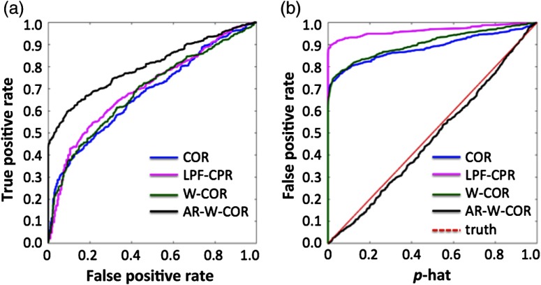
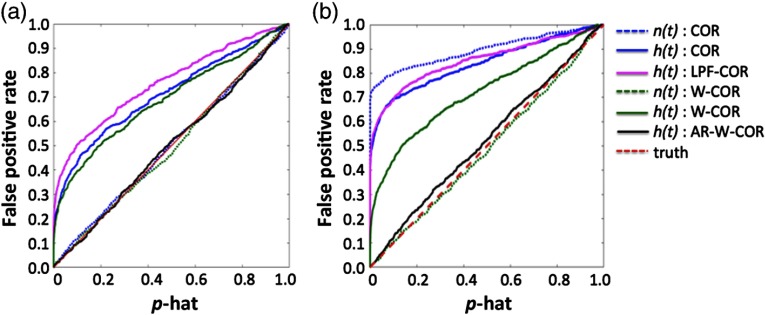
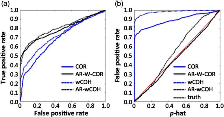
Functional near-infrared spectroscopy (fNIRS) is a noninvasive neuroimaging technique that uses low levels of red to near-infrared light to measure changes in cerebral blood oxygenation. Spontaneous (resting state) functional connectivity (sFC) has become a critical tool for cognitive neuroscience for understanding task-independent neural networks, revealing pertinent details differentiating healthy from disordered brain function, and discovering fluctuations in the synchronization of interacting individuals during hyperscanning paradigms. Two of the main challenges to sFC-NIRS analysis are (i) the slow temporal structure of both systemic physiology and the response of blood vessels, which introduces false spurious correlations, and (ii) motion-related artifacts that result from movement of the fNIRS sensors on the participants’ head and can introduce non-normal and heavy-tailed noise structures. In this work, we systematically examine the false-discovery rates of several time- and frequency-domain metrics of functional connectivity for characterizing sFC-NIRS. Specifically, we detail the modifications to the statistical models of these methods needed to avoid high levels of false-discovery related to these two sources of noise in fNIRS. We compare these analysis procedures using both simulated and experimental resting-state fNIRS data. Our proposed robust correlation method has better performance in terms of being more reliable to the noise outliers due to the motion artifacts.

Fig. 1

Demonstration of the effect of motion on fNIRS correlation analysis. In this figure, we show an example of simulated fNIRS data from two channels with a correlation of $R=0.5$ (panel a). If a motion artifact appears in one of the two channels (e.g., simulating the case where only part of the fNIRS probe moves), the motion dilutes the correlation and the connectivity is underestimated (panel b). However, if the motion artifact is co-occurring in both channels (e.g., the artifact has high spatial covariance), this can inflate the correlation and result in a high FDR (panel c) due to the strong leverage of the few affected outlier time points. (a) No motion, (b) unshared motion, and (c) shared motion.

Fig. 2

Effect of signal prewhitening on fNIRS data. Prewhitening using an autoregressive filter removes serially correlated errors in the signals. In panels (a) and (b), raw signals with no motion artifacts and with artifacts are shown. After filtering, the innovation (prewhitened) versions of these signals is shown in panels (c) and (d). This figure shows the same data presented in Fig. 1. (a) No motion (raw signal), (b) motion affected (raw signal), (c) no motion (prewhitened), (d) motion affected (prewhitened), and (e) autocorrelation.

Fig. 3

Comparison of FDR in simulated data as a result of sample rate. This figure shows the FDR for simulated “neural” $[n(t)]$ and “hemodynamic” $[h(t)]$ signals at different sampling rates and for the various correlation models described in Sec. 3.2. The expected FDR ($\alpha =0.05$) is shown in the dotted red line. Estimates above this line are considered uncontrolled type-I errors. These simulations are described in Sec. 3.1.1. The abbreviations of the methods are defined in Sec. 3.2. (a) Without motion artifacts and (b) with motion artifacts.

Fig. 4

Comparison of sensitivity–specificity in simulated data. This figure shows the sensitivity–specificity (receiver operator curves) for the various correlation models applied to the simulated “neural” $[n(t)]$ and “hemodynamic” $[h(t)]$ signals. Curves that are closer to the upper left corner have better model performance. Panels (a) and (b) show simulations in the absence and presence of motion artifacts, respectively. These simulations are described in Sec. 3.1.2. The abbreviations of the methods are defined in Sec. 3.2. (a) Without motion artifacts and (b) with motion artifacts.

Fig. 5

Comparison of sensitivity–specificity and type-I error control in experimental data. (a) The sensitivity–specificity (receiver operator curves) for the various correlation models applied to the experimental data described in Sec. 3.1.3. (b) Control for type-I errors for the same data and methods. The abbreviations of the methods are defined in Sec. 3.2.

Fig. 6

Comparison of control type-I errors in simulated data. This figure shows control for type-I errors for the various correlation models applied to the simulated “neural” $[n(t)]$ and “hemodynamic” $[h(t)]$ signals. The $y$-axis indicates the level of true false-discovery and the $x$-axis shows the reported probability ($p$-hat). An ideal curve would be along the diagonal ($\text{slope}=1$), where the reported and actual FDRs would be the same. Panels (a) and (b) show simulations in the absence and presence of motion artifacts, respectively. These simulations are described in Sec. 3.1.2. The abbreviations of the methods are defined in Sec. 3.2. (a) Without motion artifacts and (b) with motion artifacts.

Fig. 7

Comparison of sensitivity–specificity and control type-I error in experimental data. (a) Comparison of the performance of the unwhitened and prewhitened COR and wCOH models using the experimental data described in Sec. 3.1.3. (b) Control for type-I errors for the same data and methods. In panel (b), idealized control for type-I error is indicated by a line of unity slope (red dotted line). The abbreviations of the methods are defined in Sec. 3.2.

References

1. Fox M. D., Raichle M. E., “Spontaneous fluctuations in brain activity observed with functional magnetic resonance imaging,” Nat. Rev. Neurosci. 8, 700–711 (2007).10.1038/nrn2201 - DOI - PubMed
1. Greicius M., “Resting-state functional connectivity in neuropsychiatric disorders,” Curr. Opin. Neurol. 21, 424–430 (2008).10.1097/WCO.0b013e328306f2c5 - DOI - PubMed
1. Smith S. M., et al. , “Correspondence of the brain’s functional architecture during activation and rest,” Proc. Natl. Acad. Sci. U.S.A 106, 13040 (2009).10.1073/pnas.0905267106 - DOI - PMC - PubMed
1. Arieli A., et al. , “Dynamics of ongoing activity: explanation of the large variability in evoked cortical responses,” Science 273, 1868–1871 (1996).SCIEAS10.1126/science.273.5283.1868 - DOI - PubMed
1. Biswal B., et al. , “Functional connectivity in the motor cortex of resting human brain using echo-planar MRI,” Magn. Reson. Med. 34, 537–541 (1995).10.1002/(ISSN)1522-2594 - DOI - PubMed