. 2017 May 15;15(1):41.
doi: 10.1186/s12915-017-0377-3.

OptiMouse: a comprehensive open source program for reliable detection and analysis of mouse body and nose positions

Affiliations

OptiMouse: a comprehensive open source program for reliable detection and analysis of mouse body and nose positions

Yoram Ben-Shaul. BMC Biol. .

Abstract

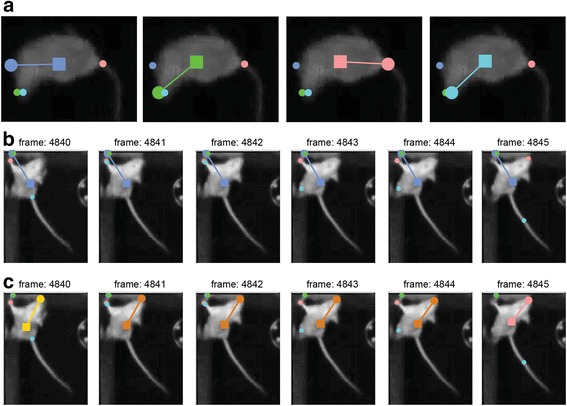
Background: Accurate determination of mouse positions from video data is crucial for various types of behavioral analyses. While detection of body positions is straightforward, the correct identification of nose positions, usually more informative, is far more challenging. The difficulty is largely due to variability in mouse postures across frames.

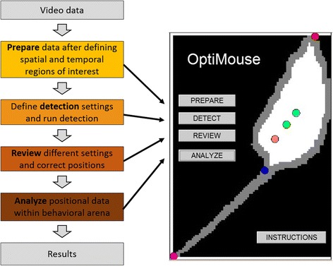
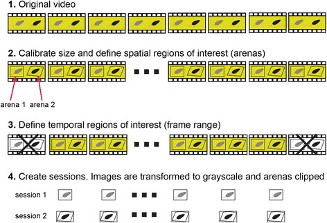
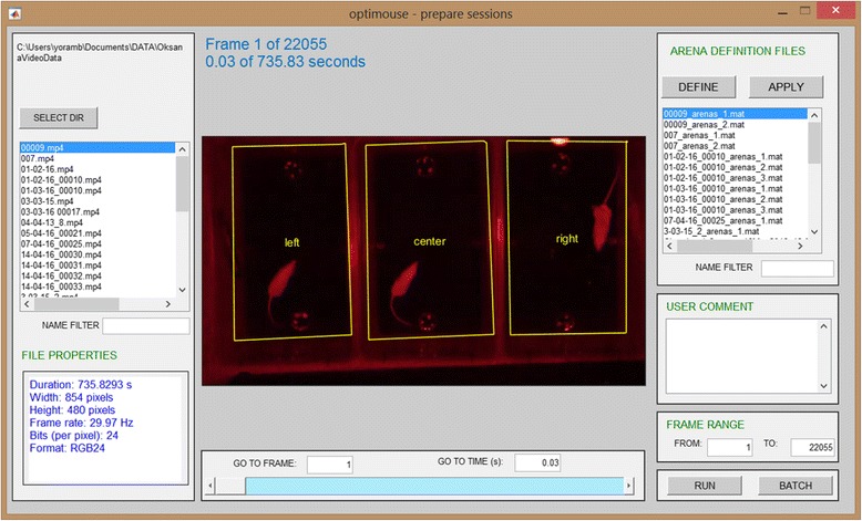
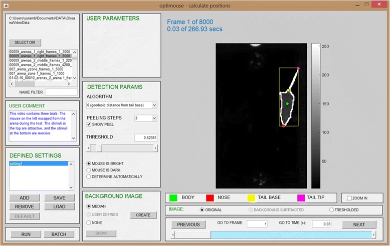
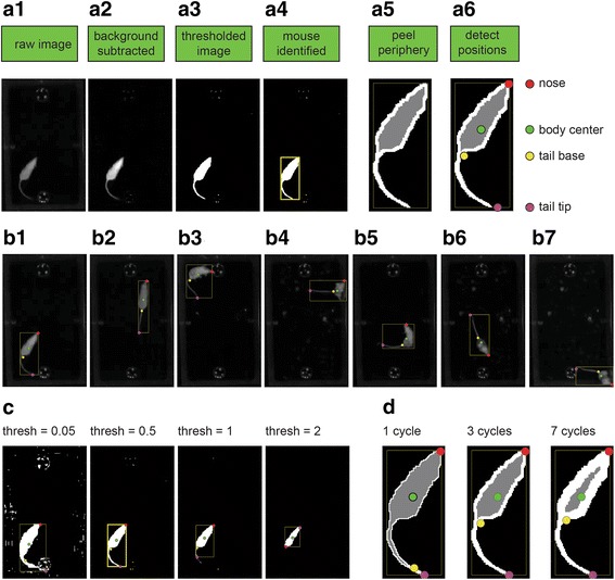
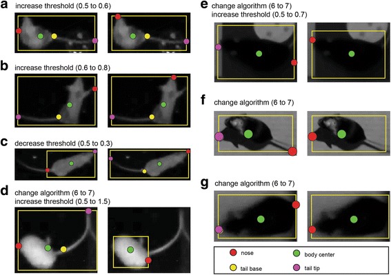
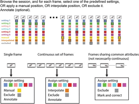
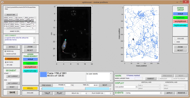
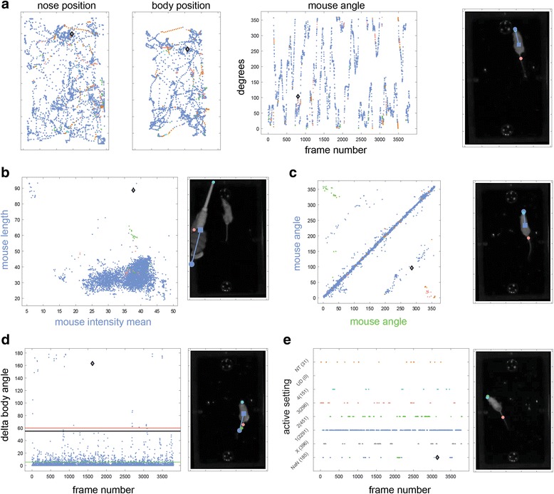
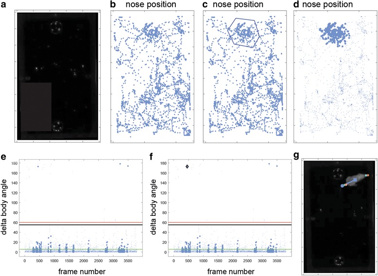
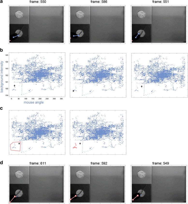
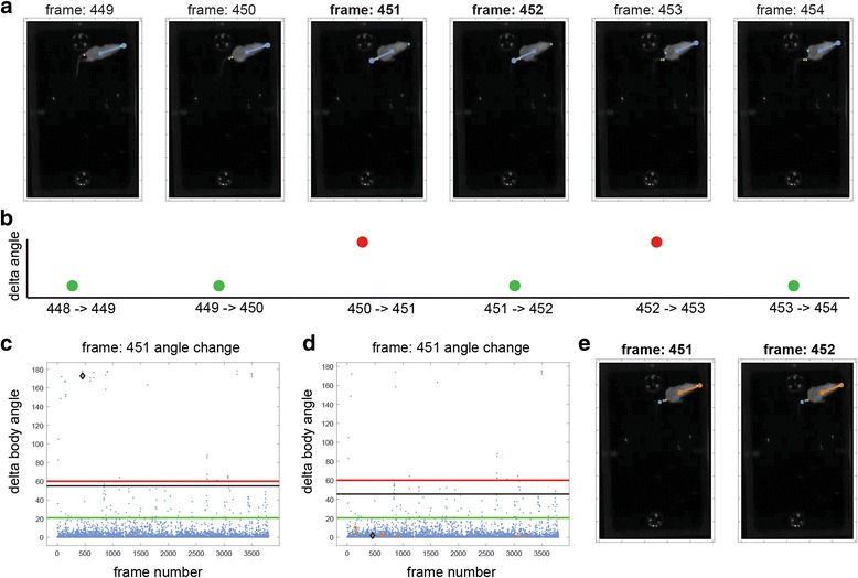
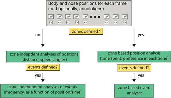
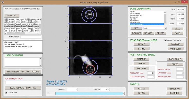
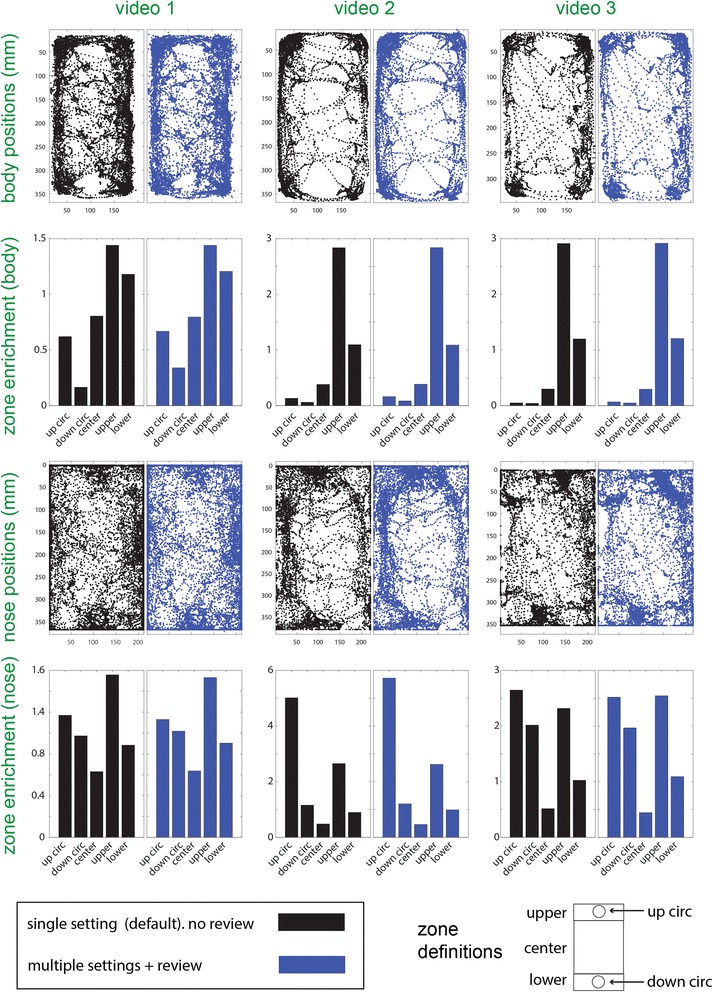
Results: Here, we present OptiMouse, an extensively documented open-source MATLAB program providing comprehensive semiautomatic analysis of mouse position data. The emphasis in OptiMouse is placed on minimizing errors in position detection. This is achieved by allowing application of multiple detection algorithms to each video, including custom user-defined algorithms, by selection of the optimal algorithm for each frame, and by correction when needed using interpolation or manual specification of positions.

Conclusions: At a basic level, OptiMouse is a simple and comprehensive solution for analysis of position data. At an advanced level, it provides an open-source and expandable environment for a detailed analysis of mouse position data.

Keywords: Position analysis; Preference tests; Rodent behavior; Video data.


Figures

Fig. 1.
Fig. 1.
The main modules in OptiMouse. The left side shows a workflow of the main analysis stages. The right image shows the main OptiMouse interface. Each of the four buttons evokes a GUI for the corresponding stage
Fig. 2.
Fig. 2.
Schematic description of the session preparation process. Preparation involves spatial definitions of one or more arenas and size calibration as well as optional removal of irrelevant video sections. Video data for each of the sessions is converted to grayscale images
Fig. 3.
Fig. 3.
The Prepare GUI. The Prepare GUI is shown after definition of three arenas (named left, center, and right). The GUI for arena definition is accessed via the Define button (see the manual for details)
Fig. 4.
Fig. 4.
Schematic of the detection stage. In very broad terms, one or more detection settings (up to six) are applied to each of the frames of the video. Each setting involves several user defined parameters and potentially also user specified algorithms. The selection among the various settings is applied in the review stage
Fig. 5.
Fig. 5.
The Detect GUI. The Detect GUI is shown with one setting defined
Fig. 6.
Fig. 6.
The detection process. a The key stages of nose and body detection. b Examples of detection of various frames in a single session. c Effects of changing the detection threshold. d Effects of changing the number of peeling cycles
Fig. 7.
Fig. 7.
Examples of incorrect detection (left image in each panel) and their correction (right images). Some detection failures can be fixed by adjusting the detection threshold (i.e., ac) but others require more extensive adjustments. In (d), the mouse is grooming its tail, with the nose positioned close to the tail base. Such cases are difficult to detect consistently in static images, but are apparent when viewed in the context of a movie. Although it is easy to modify the parameters to achieve correct detection in this frame, it is challenging to generate an algorithm that will reliably identify the nose under such cases. In some cases, application of another algorithm is required. For example, algorithm 7 (Additional file 1) is suitable when the tail is not included in the thresholded image. This indeed is the remedy for the examples in (dg), sometimes combined with a modified threshold. In (f), the left image shows an obvious failure with the tail detected as nose. Detection is improved when the algorithm is changed, yet is still not perfect, since the shadow cast by the nose is detected as the nose. This problem is also beyond the scope of the built-in algorithms, as the shadow is darker than the nose and just as sharp
Fig. 8.
Fig. 8.
A schematic overview of the reviewing stage. This graphic on top illustrates the operations that can be applied to each frame. The bottom panels show that such operations can be applied to individual frames, to a continuous segment of frames, and to frames sharing common attributes
Fig. 9.
Fig. 9.
The review GUI. The review GUI is shown after four settings have been defined during the detection stage
Fig. 10.
Fig. 10.
Examples illustrating the application of detection settings. a Application of different (predefined) settings to a single frame. The active setting is indicated by a larger circle denoting the nose position, a square denoting the body center, and a line connecting them. In the leftmost frame, the active setting is the default (first) setting. In each of the other frames, there is a different active setting. b A sequence of frames with incorrect detection. In this example, the default method fails for the entire segment of frames. c The solution involves three stages. First, a manual position, indicated in yellow, is defined for the first frame in the sequence (4840). Next, setting 3 (pink), is applied to the last frame in the sequence (4845). Finally, the set of frames is defined as a segment (Additional file 1), and the positions within it are interpolated. The interpolated positions are shown in ochre (frames 4841-4844). See the manual for a detailed description of the two available interpolation algorithms
Fig. 11.
Fig. 11.
Examples of some parameter views. In all cases, the current frame is indicated by a diamond, and is shown to the right of each view. a Views associated with position. b Length verus mean intensity of the detected object. c Comparison of angles detected by each of the two settings. The settings which apply to each axis are indicated by the label colors (blue and green denoting the first and second settings, respectively). d View showing body angle change as a function of frame number. Extreme change values, as shown in this example, often reveal erroneous detections. e View showing the setting associated with each frame
Fig. 12.
Fig. 12.
Procedure for marking frames with particular attributes. In this example, frames associated with particular nose positions are marked, and then examined for abrupt changes in direction. a One frame showing positions of odor plates in the arena. b View showing nose positions before marking. c Same view during the process of marking a subset of frames near upper odor plate. d In this view, the marked frames are highlighted. e After switching to a different view, the marked frames are still highlighted. In the present example, this allows identification of frames that are both associated with particular positions and with high values of body angle changes. f Selection of one such dot reveals a frame in which the mouse is near the upper plate and the tail is mistaken for the nose (g)
Fig. 13.
Fig. 13.
Applying a setting to a set of frames. a Three frames that show a similar failure of the first setting cluster together in this view (b). Applying a different setting to all these frames using a polygon (c), also corrects detection in other frames in the cluster (d)
Fig. 14.
Fig. 14.
Automatic correction of position detection errors. a Sequence of frames with a transient detection failure. b Schematic of angle changes in the sequence of frames; the magnitude of angle changes is shown qualitatively. c Actual angle changes before correction. d Angle changes after correction. e Interpolated positions in the two frames that were initially associated with errors
Fig. 15.
Fig. 15.
Schematic of possible types of analysis. Flow chart provides a very general description of possible analyses. Results can be shown as figures, saved as MATLAB data files, and for some analyses, displayed on the command prompt
Fig. 16.
Fig. 16.
The Analysis GUI after the eight zones were defined
Fig. 17.
Fig. 17.
Examples of some graphical analyses. a The arena with eight zones defined (same zones shown in Fig. 16). b Tracks defined by the body center. Colored zones indicate zone entries. Dots representing positions assume colors of corresponding zones. c Tracks made by the nose. d Heatmap of zone positions. e Zone occupancy as a function of time. Each row corresponds to one of the zones. When the nose is inside a specific zone at a particular frame, this is indicated by a dot. Dots in this display are so dense that they appear as lines. f Enrichment score (of the nose) as a function of time. g Total nose time in each zone. h Enrichment score at the end of the session
Fig. 18.
Fig. 18.
Comparison of positional analysis with and without reviewing for three different videos. Each video is shown in one column, and each row represents one type of analysis. The first row from the top shows body position coordinates. The second row shows enrichment scores of body positions in each of five different zones, whose coordinates relative to the arena are shown at the bottom of the figure. The third and fourth rows from the top are similar to the upper rows, except that nose, rather than body positions, are shown. Each panel contains two plots. The plots on the left (in black) show the results using the default setting, while plots on the right (blue) show the same analyses after the application of non-default settings, including manual settings

Comment in

  • Knowing where the nose is.
    Gillis WF, Datta SR. Gillis WF, et al. BMC Biol. 2017 May 15;15(1):42. doi: 10.1186/s12915-017-0382-6. BMC Biol. 2017. PMID: 28506236 Free PMC article.

References

    1. da Lin Y, Zhang SZ, Block E, Katz LC. Encoding social signals in the mouse main olfactory bulb. Nature. 2005;434(7032):470–7. doi: 10.1038/nature03414. - DOI - PubMed
    1. Cichy A, Ackels T, Tsitoura C, Kahan A, Gronloh N, Sochtig M, et al. Extracellular pH regulates excitability of vomeronasal sensory neurons. J Neurosci. 2015;35(9):4025–39. doi: 10.1523/JNEUROSCI.2593-14.2015. - DOI - PMC - PubMed
    1. Root CM, Denny CA, Hen R, Axel R. The participation of cortical amygdala in innate, odour-driven behaviour. Nature. 2014;515(7526):269–73. doi: 10.1038/nature13897. - DOI - PMC - PubMed
    1. Ferrero DM, Lemon JK, Fluegge D, Pashkovski SL, Korzan WJ, Datta SR, et al. Detection and avoidance of a carnivore odor by prey. Proc Natl Acad Sci U S A. 2011;108(27):11235–40. doi: 10.1073/pnas.1103317108. - DOI - PMC - PubMed
    1. Brock O, Bakker J, Baum MJ. Assessment of urinary pheromone discrimination, partner preference, and mating behaviors in female mice. Methods Mol Biol. 2013;1068:319–29. doi: 10.1007/978-1-62703-619-1_24. - DOI - PubMed

Publication types