Linkage disequilibrium matches forensic genetic records to disjoint genomic marker sets

Abstract

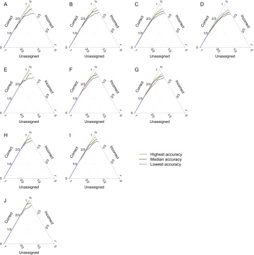
Combining genotypes across datasets is central in facilitating advances in genetics. Data aggregation efforts often face the challenge of record matching-the identification of dataset entries that represent the same individual. We show that records can be matched across genotype datasets that have no shared markers based on linkage disequilibrium between loci appearing in different datasets. Using two datasets for the same 872 people-one with 642,563 genome-wide SNPs and the other with 13 short tandem repeats (STRs) used in forensic applications-we find that 90-98% of forensic STR records can be connected to corresponding SNP records and vice versa. Accuracy increases to 99-100% when ∼30 STRs are used. Our method expands the potential of data aggregation, but it also suggests privacy risks intrinsic in maintenance of databases containing even small numbers of markers-including databases of forensic significance.

Keywords: forensic DNA; genomic privacy; imputation; population genetics; record matching.

Fig. 1.

Allelic imputation accuracies for 13 CODIS loci. The figure shows imputation accuracy for the partition of 872 individuals into training (75%) and test (25%) sets that yielded median (51st greatest) record-matching accuracy by the Hungarian method among 100 partitions. Beagle accuracy is obtained by imputing the STR genotype assigned the highest imputation probability by Beagle. Null accuracy is obtained by imputing the same high-frequency STR genotype in all individuals regardless of nearby SNP genotypes. Vertical lines represent 95% confidence intervals based on 10,000 bootstrap resamples of individuals from the test set. Beagle accuracies are significantly higher (Wilcoxon signed rank test, two-tailed p < 0.05) than null accuracies at all loci except one (D18S51; p = 0.09). Beagle accuracy is also higher when measuring total numbers of alleles imputed correctly in each person (p < 2.2 × 10⁻¹⁶). Beagle and null accuracies are negatively correlated with heterozygosities reported in Table S2.

Fig. S1.

Allelic imputation accuracies for 431 non-CODIS tetranucleotide STR loci. The plot considers the partition of the data represented in Fig. 1. Beagle imputation accuracy is obtained by imputing the STR genotype assigned the highest imputation probability by Beagle. Null imputation accuracy is obtained by imputing the same STR genotype for all people, irrespective of nearby SNP genotypes. Markers are sorted from left to right by null accuracy. Across all loci, the mean null accuracy is 0.497, and the mean Beagle accuracy is 0.624. Note that ref. compared 432 rather than 431 non-CODIS tetranucleotides with the CODIS loci; we omitted TPO-D2S, an alias for the CODIS locus TPOX.

Fig. 2.

Match scores of records that truly match and match scores of nonmatches. (A) The matrix of match scores (Eq. 1) comparing 218 CODIS STR profiles with 218 SNP profiles for the data partition represented in Fig. 1. Each cell gives a match score for the pairing of a SNP profile with a CODIS profile. Scores pairing a given CODIS profile with each SNP profile appear in a column, and scores pairing a given SNP profile with each CODIS profile appear in a row. Darker colors represent larger values. Population memberships are colored by geographic region: Africa, orange; Europe, blue; Middle East, yellow; Central/South Asia, red; East Asia, pink; Oceania, green; Americas, purple). Of 52 populations in our dataset (Table S1), 47 appear in the test set shown. True matches are on a diagonal from the bottom left to the top right, and they tend to have higher match scores than off-diagonal nonmatches. Population structure is also visible (Table S3). For example, SNP profiles from Africans tend to have low match scores with non-Africans, and match scores of nonmatches tend to be higher when both CODIS and SNP profiles are from Native Americans. (B) Kernel density estimate for match scores. We applied a normal kernel with bandwidth chosen by Silverman’s rule (option nrd0 in the density function in R) to the matrix entries in A. Nonmatches tend to have negative log-likelihood match scores, whereas true matches tend to have positive scores.

Fig. 3.

The proportions of profiles unassigned, correctly assigned, and incorrectly assigned as the match-score threshold is varied. When the threshold is large, all profiles are unassigned (lower left vertex). Gradually lowering the threshold leads to assignment of all profiles, tracing a curve to the right edge. Of 100 partitions into training and test sets, the figure plots trials with maximum, median, and minimum accuracies when all possible profiles are paired. (A) One-to-one matching. (B) One-to-many matching selecting the STR profile that best matches a query SNP profile. (C) One-to-many matching selecting the SNP profile that best matches a query STR profile. (D) Needle-in-haystack matching counting the proportion of true matches with match score that exceeds the maximal match score among nonmatches. In D, after the match-score threshold is lower than the largest match score among nonmatches, all pairings are marked incorrect.

Fig. S2.

The median proportion of test-set CODIS and SNP records matched correctly as a function of the sizes of the training and test sets. We divided the data into training and test sets in 1,000 ways, examining training sets of sizes 436, 545, 654, and 763—representing 50, 62.5, 75, and 87.5% of the data. For each training-set size, we used test-set sizes that were multiples of 109 (1/8 of 872), so that the sum of training-set and test-set sizes did not exceed 872. For each of 10 possible schemes for the proportions representing the training and test sets, we considered 100 random divisions of the data, using the same 100 partitions in all analyses for a given scheme. (A) One-to-one matching. (B) One-to-many matching selecting the STR profile that best matches a query SNP profile. (C) One-to-many matching selecting the SNP profile that best matches a query STR profile. (D) Needle-in-haystack matching. In D, the vertical axis has the same scale as in the other panels.

Fig. S3.

Proportions of the sample unassigned, correctly assigned, and incorrectly assigned as a function of the match-score threshold under one-to-one matching using the Hungarian method. Each panel considers different proportions (training, test) of the total data (n = 872) allocated into training and test sets, with 100 allocations according to those proportions. (A) 1/2, 1/8. (B) 1/2, 1/4. (C) 1/2, 3/8. (D) 1/2, 1/2. (E) 5/8, 1/8. (F) 5/8, 1/4. (G) 5/8, 3/8. (H) 3/4, 1/8. (I) 3/4, 1/4. (J) 7/8, 1/8. The figure design follows Fig. 3.

Fig. S4.

The median value of the mean allelic imputation accuracy across 13 CODIS markers as a function of the size of the training set. Beagle and null imputation accuracies follow Fig. 1. The median is taken across 100 partitions into training and test sets. Imputation accuracies are plotted for all 10 schemes for the sizes of training and test sets; multiple test-set sizes produce similar values at a fixed training-set size, and they are represented by overlapping plotted points. The lines connect the median values for the test-set sizes at given training-set sizes.

Fig. S5.

Proportions of the sample unassigned, correctly assigned, and incorrectly assigned as a function of the match-score threshold under one-to-many matching that attempts to find the CODIS profile that matches a query SNP profile. Each panel considers different proportions (training, test) of the total data (n = 872) allocated into training and test sets, with 100 allocations according to those proportions. (A) 1/2, 1/8. (B) 1/2, 1/4. (C) 1/2, 3/8. (D) 1/2, 1/2. (E) 5/8, 1/8. (F) 5/8, 1/4. (G) 5/8, 3/8. (H) 3/4, 1/8. (I) 3/4, 1/4. (J) 7/8, 1/8. The figure design follows Fig. 3.

Fig. S6.

Proportions of the sample unassigned, correctly assigned, and incorrectly assigned as a function of the match-score threshold under one-to-many matching that attempts to find the SNP profile that matches a query CODIS profile. Each panel considers different proportions (training, test) of the total data (n = 872) allocated into training and test sets, with 100 allocations according to those proportions. (A) 1/2, 1/8. (B) 1/2, 1/4. (C) 1/2, 3/8. (D) 1/2, 1/2. (E) 5/8, 1/8. (F) 5/8, 1/4. (G) 5/8, 3/8. (H) 3/4, 1/8. (I) 3/4, 1/4. (J) 7/8, 1/8. The figure design follows Fig. 3.

Fig. S7.

Proportions of the sample unassigned, correctly assigned, and incorrectly assigned as a function of the match-score threshold under needle-in-haystack matching. Each panel considers different proportions (training, test) of the total data (n = 872) allocated into training and test sets, with 100 allocations according to those proportions. (A) 1/2, 1/8. (B) 1/2, 1/4. (C) 1/2, 3/8. (D) 1/2, 1/2. (E) 5/8, 1/8. (F) 5/8, 1/4. (G) 5/8, 3/8. (H) 3/4, 1/8. (I) 3/4, 1/4. (J) 7/8, 1/8. The figure design follows Fig. 3.

Fig. 4.

Record-matching accuracy as a function of number of STRs. For each number of loci, 100 random locus sets are analyzed for the data partition in Fig. 1; results are shown horizontally jittered. (A) One-to-one matching. (B) One-to-many matching selecting the STR profile that best matches a query SNP profile. (C) One-to-many matching selecting the SNP profile that best matches a query STR profile. (D) Needle-in-haystack matching.

References

1. de Bakker PI, et al. Practical aspects of imputation-driven meta-analysis of genome-wide association studies. Hum Mol Genet. 2008;17:R122–R128. - PMC - PubMed
1. Li Y, Willer C, Sanna S, Abecasis G. Genotype imputation. Annu Rev Genomics Hum Genet. 2009;10:387–406. - PMC - PubMed
1. Marchini J, Howie B. Genotype imputation for genome-wide association studies. Nat Rev Genet. 2010;11:499–511. - PubMed
1. Presson AP, Sobel E, Lange K, Papp JC. Merging microsatellite data. J Comput Biol. 2006;13:1131–1147. - PubMed
1. Pemberton TJ, DeGiorgio M, Rosenberg NA. Population structure in a comprehensive genomic data set on human microsatellite variation. G3 (Bethesda) 2013;3:891–907. - PMC - PubMed
Publication types
MeSH terms
Substances
LinkOut - more resources