High Arctic Holocene temperature record from the Agassiz ice cap and Greenland ice sheet evolution

Abstract

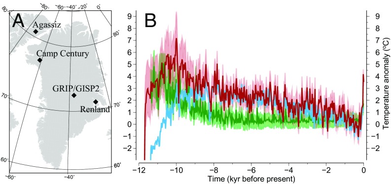
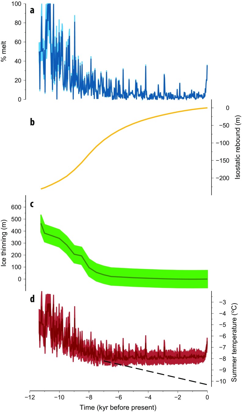
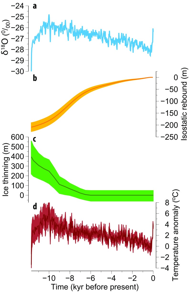
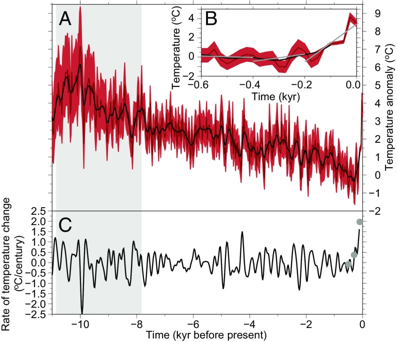
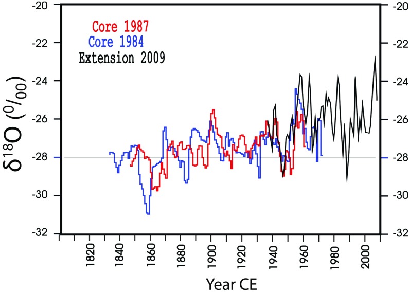
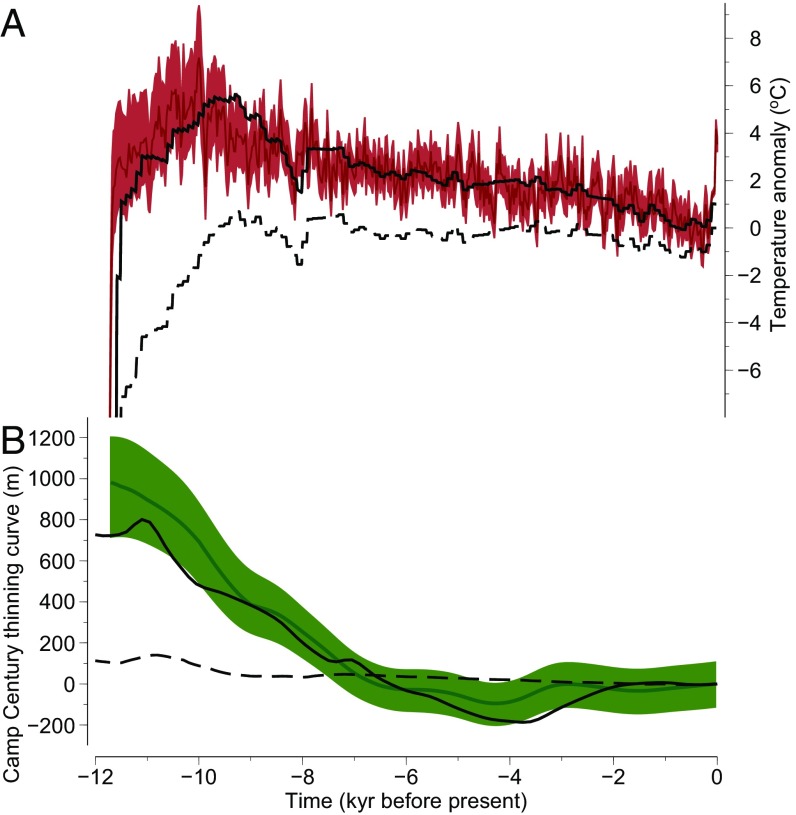
We present a revised and extended high Arctic air temperature reconstruction from a single proxy that spans the past ∼12,000 y (up to 2009 CE). Our reconstruction from the Agassiz ice cap (Ellesmere Island, Canada) indicates an earlier and warmer Holocene thermal maximum with early Holocene temperatures that are 4-5 °C warmer compared with a previous reconstruction, and regularly exceed contemporary values for a period of ∼3,000 y. Our results show that air temperatures in this region are now at their warmest in the past 6,800-7,800 y, and that the recent rate of temperature change is unprecedented over the entire Holocene. The warmer early Holocene inferred from the Agassiz ice core leads to an estimated ∼1 km of ice thinning in northwest Greenland during the early Holocene using the Camp Century ice core. Ice modeling results show that this large thinning is consistent with our air temperature reconstruction. The modeling results also demonstrate the broader significance of the enhanced warming, with a retreat of the northern ice margin behind its present position in the mid Holocene and a ∼25% increase in total Greenland ice sheet mass loss (∼1.4 m sea-level equivalent) during the last deglaciation, both of which have implications for interpreting geodetic measurements of land uplift and gravity changes in northern Greenland.

Keywords: Greenland ice sheet; Holocene climate; ice core; temperature reconstruction.

Fig. 1.

Location map and Agassiz proxy temperature records: (A) Map showing the study area with the names and locations of ice core borehole sites mentioned in the text. (B) The 25-y resolution, elevation-corrected Agassiz δ¹⁸O temperature reconstruction (dark red) with 2σ uncertainty (light red) and the elevation-corrected Agassiz melt record (green), both extended to 2009 CE. Ref. ’s δ¹⁸O Agassiz–Renland temperature reconstruction is also shown (blue) for comparison. Each record is referenced to its preindustrial temperature value at 1750 CE.

Fig. S1.

Empirical melt percent transfer function: Summer temperatures and melt layers across a number of shallow Arctic ice cores (black circles; refs. 7, 30). Linear regression of these data yield a transfer function (black line; 2σ is the dashed black line), which demonstrates that summer temperatures below ∼−8 °C yield no melt fraction in the ice. Similarly, melt percent values of 100 signify summer temperatures above or equal to ∼−3 °C.

Fig. 2.

Various records related to high Arctic climate change: (A) Agassiz δ¹⁸O temperature reconstruction (dark red) with its 2σ uncertainty (light red). (B) Agassiz melt record summer (JJA) temperature reconstruction with the potential trend (dashed black) for temperatures below −8 °C and above −3 °C (horizontal gray dash; see main text and Methods). (C) Mean annual insolation at 80°N. (D) Agassiz tree (purple) and herb (pink) pollen record (15), (E) sea salt sodium in the GISP2 (doubled scaling; cyan; ref. 17) and Penny ice cores (green; ref. 16), and (F) numbers of bowhead whale bones from Eastern (gray; 74.3–76.1°N, 83.3–90.5°W; n = 116) and Central (black; 71.5–73.7°N, 89.4–99.0°W; n = 96) Queen Elizabeth Islands (18, 19). The gray area denotes the local Holocene thermal maximum, a period when Agassiz temperatures were regularly above peak contemporary values.

Fig. S2.

Agassiz melt-record temperature reconstruction: (A) Agassiz melt record and estimated corrections for (B) isostatic adjustment and (C) thinning of the Innuitian ice sheet at the borehole site. (D) The resulting summer (JJA) temperature reconstruction (dark red) with its 2σ uncertainty (light red). The potential mid to late Holocene trend for temperatures below −8 °C (when there is absence of melt) is indicated by the dashed black line.

Fig. S3.

Agassiz δ¹⁸O temperature reconstruction: (A) Agassiz δ¹⁸O record with the addition of the 2010 shallow ice core and estimated elevation corrections for (B) isostatic adjustment and (C) thinning of the Innuitian ice sheet along the southeastern coast of Ellesmere Island. (D) Agassiz δ¹⁸O temperature reconstruction (dark red) with its 2σ uncertainty (light red).

Fig. 3.

Low-pass-filtered Agassiz δ¹⁸O temperature reconstruction: (A) Agassiz δ¹⁸O temperature reconstruction (dark red) with its 2σ uncertainty (light red) with the Gaussian filtered (σ = 50 y) reconstruction (black). (B) The Agassiz δ¹⁸O temperature reconstruction over the past 1,000 y. The gray lines denote the linear regression results for three periods: the cooling leading into the preindustrial period, the preindustrial era, and industrial era. (C) Rate of temperature change (black) based on the Gaussian filtered Agassiz temperature reconstruction. The gray circles represent the rates of change obtained from the linear regression segments shown in B. The vertical gray band denotes the local Holocene thermal maximum, a period when Agassiz temperatures were regularly above peak contemporary values.

Fig. S4.

Agassiz δ¹⁸O extension: A84, A87, and A09 high resolution δ(¹⁸O) series. In the overlap period approximately from 1940 to 1970 CE, there is reasonable correlation and good matching of levels. The differences between the three series are typical for such high-resolution series at this latitude (8).

Fig. 4.

Temperature and thinning curves for northwest Greenland: (A) Agassiz δ¹⁸O temperature reconstruction (dark red) with 2σ uncertainty (light red). The temperature time series at Camp Century inferred from the GRIP ice core using a δ¹⁸O–temperature relationship and lapse rate correction (dashed black) and the revised temperature time series based on the Agassiz reconstruction (solid black; Methods). (B) Camp Century thinning curve (green) and 2σ uncertainty (light green) compared with model output: Huy3 (dashed black) and our variant of this model reconstruction (solid black).

Fig. S5.

Camp Century thinning history: Camp Century ice-core-derived Holocene thinning curves from ref. (blue) and this study (orange); light band represents the 2σ uncertainty range. Selected model predictions are shown in dashed gray (31), gray (32), dashed black (22), and black (this study).

Fig. S6.

Relative sea level and GPS sites: The location of the relative sea level sites shown in Fig. S7 are indicated by downward-facing triangles. The diamonds represent the locations of the Agassiz and Camp Century ice cores. The circles represent the locations of the Greenland GPS Network (GNET) sites in North Greenland listed in Table S1.

Fig. S7.

Relative sea level data and predictions: RSL data and model predictions based on two ice models: Huy3 (dashed black) and the variant of Huy3 from this study (solid black). Lower relative sea-level limiting dates are denoted by blue upward-pointing triangles and upper limiting dates are shown by red downward-pointing triangles. The gray dashed horizontal line represents the marine limit, which marks the highest point reached by sea level during ice-free conditions at each location. Location map of sites is shown in Fig. S6.

Fig. S7.

Relative sea level data and predictions: RSL data and model predictions based on two ice models: Huy3 (dashed black) and the variant of Huy3 from this study (solid black). Lower relative sea-level limiting dates are denoted by blue upward-pointing triangles and upper limiting dates are shown by red downward-pointing triangles. The gray dashed horizontal line represents the marine limit, which marks the highest point reached by sea level during ice-free conditions at each location. Location map of sites is shown in Fig. S6.

Fig. S8.

Modeled ice volume of the GrIS: Huy3 and variant reconstruction volume histories shown as dashed black and solid black curves, respectively. The differences between the two volume histories are due to changes in North Greenland associated with the revised climate forcing.

Fig. S9.

Modeled ice sheet rates of change during the Holocene: (A) Rate of elevation change at Camp Century in the Huy3 variant reconstruction and (B) Greenland-wide mass balance rates.

References

1. Stocker TF, et al. IPCC, 2013: Climate Change 2013: The Physical Science Basis. Contribution of Working Group I to the Fifth Assessment Report of the Intergovernmental Panel on Climate Change. Cambridge Univ Press; Cambridge: 2013.
1. Marcott SA, Shakun JD, Clark PU, Mix AC. A reconstruction of regional and global temperature for the past 11,300 years. Science. 2013;339:1198–1201. - PubMed
1. Masson-Delmotte V, et al. Climate Change 2013: The Physical Science Basis. Contribution of Working Group I to the Fifth Assessment Report of the Intergovernmental Panel on Climate Change. Cambridge Univ Press; Cambridge: 2013. Information from paleoclimate archives; pp. 383–464.
1. Bekryaev RV, Polyakov IV, Alexeev VA. Role of polar amplification in long-term surface air temperature variations and modern arctic warming. J Clim. 2010;23:3888–3906.
1. Vinther BM, et al. Holocene thinning of the Greenland ice sheet. Nature. 2009;461:385–388. - PubMed
Publication types
LinkOut - more resources