Transformation of Cortex-wide Emergent Properties during Motor Learning

Abstract

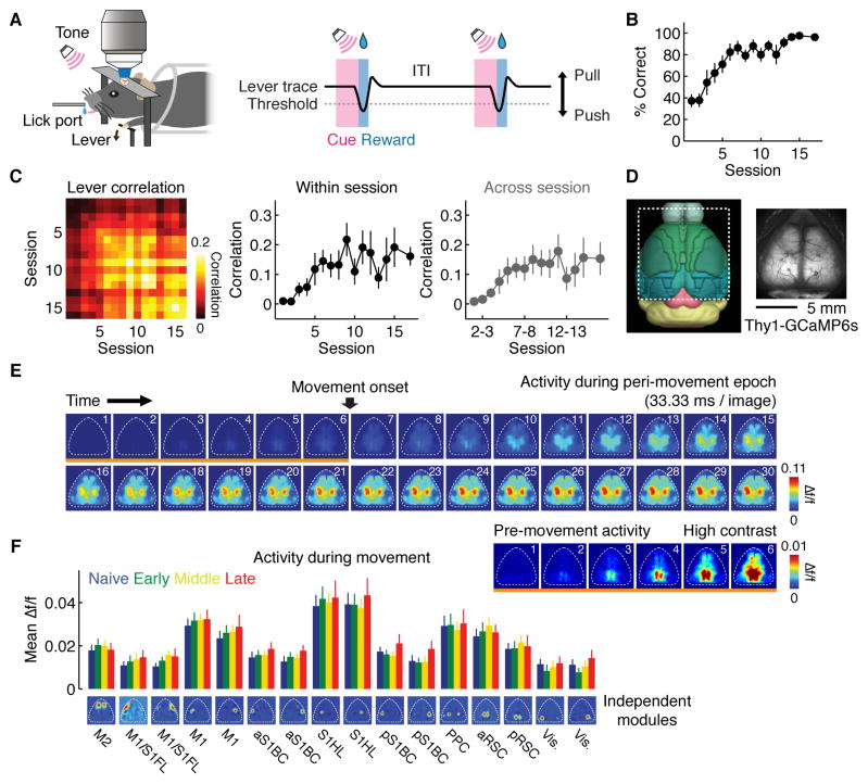
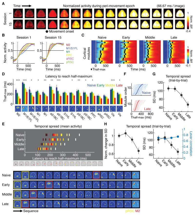
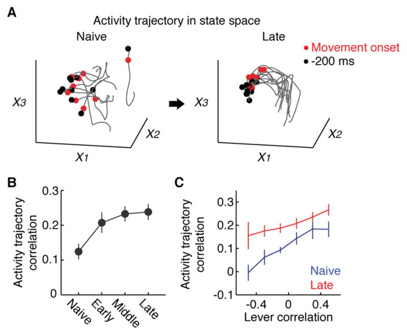
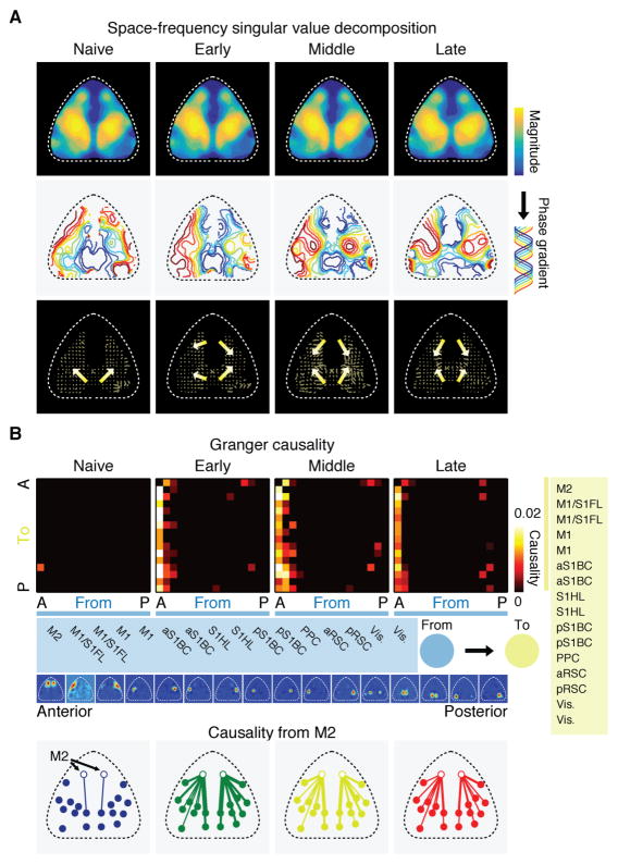
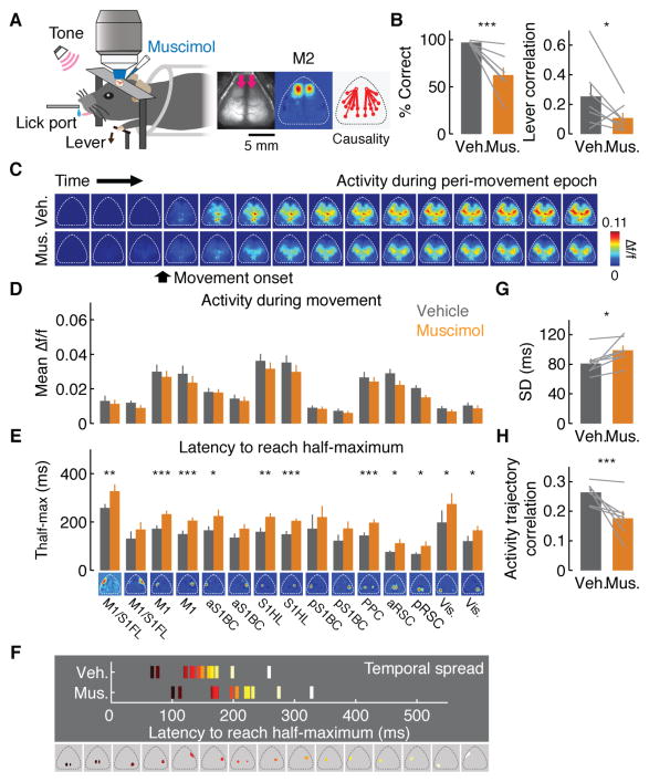
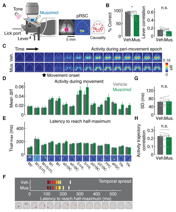
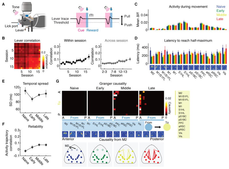
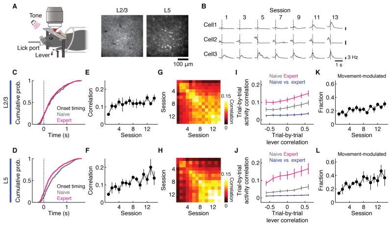
Learning involves a transformation of brain-wide operation dynamics. However, our understanding of learning-related changes in macroscopic dynamics is limited. Here, we monitored cortex-wide activity of the mouse brain using wide-field calcium imaging while the mouse learned a motor task over weeks. Over learning, the sequential activity across cortical modules became temporally more compressed, and its trial-by-trial variability decreased. Moreover, a new flow of activity emerged during learning, originating from premotor cortex (M2), and M2 became predictive of the activity of many other modules. Inactivation experiments showed that M2 is critical for the post-learning dynamics in the cortex-wide activity. Furthermore, two-photon calcium imaging revealed that M2 ensemble activity also showed earlier activity onset and reduced variability with learning, which was accompanied by changes in the activity-movement relationship. These results reveal newly emergent properties of macroscopic cortical dynamics during motor learning and highlight the importance of M2 in controlling learned movements.

Keywords: emergent properties; macroscopic cortical circuit; motor learning; premotor cortex; two-photon calcium imaging; wide-field calcium imaging.

Figure 1. Behavior and wide-field calcium imaging

(A) Left, experimental setup. Right, task structure. ITI, inter-trial interval. (B) Behavioral performance (p < 0.001, n = 8 mice, Kruskal-Wallis test, mean ± SEM). The last time point is the average of 3 sessions after the 15th session. (C) Left, correlation matrix of the lever trajectory in individual trials. Each box represents the median of all pairwise trial-by-trial correlations of movements from within or across sessions. Middle, trial-by-trial correlations of the lever trajectory within each session, corresponding to the central diagonal in the matrix on left (p < 0.01, n = 8 mice, Kruskal-Wallis test, mean ± SEM). Right, trial-by-trial correlations of the lever trajectory across adjacent sessions (p < 0.05, n = 8 mice, Kruskal-Wallis test, mean ± SEM). (D) Field of view of wide-field calcium imaging in the mouse cortex expressing GCaMP6s under the Thy1 promoter (GP4.3 line). Left panel was obtained from the Brain Explorer 2 (Allen Institute for Brain Science). (E) Example of Δf/f during the peri-movement epoch trial-averaged in a single session (between −200 ms and +800 ms relative to the movement onset). Bottom right panel shows the images indicated by the orange underline with a different contrast, highlighting that activity in some areas start before movement onset. (F) Amplitude of movement-related activity at each learning stage, measured by mean Δf/f between 0 ms and +800 ms relative to the movement onset (n.s. for all cortical modules, p > 0.05, n = 8 mice, regression, mean ± SEM).

Figure 2. Temporal compression of sequential activity across cortical modules

(A) Mean peri-movement activity across animals in sessions 1 and 15, illustrating the enhanced speed of activity after learning. Each pixel was normalized to its maximum after subtraction of activity at movement onset. (B) Mean peri-movement activity in different cortical modules in sessions 1 and 15 in aligned to movement onset (0 ms). Each module was normalized to its peak after subtraction of activity at movement onset. The time point where each line crosses the horizontal line corresponds to the time to reach half-maximum (T_half-max). (C) Mean activity across all animals in each learning stage. Activity was averaged across animals and then normalized. Black bars indicate T_half-max. Cortical modules were sorted in the antero-posterior direction. (D) T_half-max of 16 cortical modules at each learning stage (***p < 0.001, **p < 0.01, *p < 0.05, n = 8 mice, regression, corrected for multiple comparisons by false discovery rate, mean ± SEM). Naive, session 1; Early, sessions 3, 5 and 7; Middle, sessions 11, 13 and 15; Late, sessions 16–18. (E) Top, mean T_half-max of 16 cortical modules colored based on the order at the naive stage (bottom). Activity sequence becomes temporally compressed with learning. Bottom, activity sequence based on the mean T_half-max of 16 cortical modules. pRSC and M2 are highlighted by yellow and red boxes, respectively. (F) Example of sorted activity sequences from 50 randomly selected trials from naive and late stages. (G) Temporal compression of sequential activity over learning, measured by a reduction in the standard deviation of T_half-max across 16 cortical modules in individual trials (p < 0.001, n = 8 mice, regression, mean ± SEM). (H) Left, temporal compression of sequential activity is not due to changes in movement speed. Given the same movement speed, the temporal compression of sequential activity was still observed over learning (p < 0.01, n = 8 mice, regression, mean ± SEM). Trials were binned according to movement speed across sessions and the activity spread was measured in each bin at each learning stage (STAR Methods). These values were then normalized to the value of the same bin at the naive stage and averaged within bins. Right, temporal compression of sequential activity is not due to changes in movement correlation. Given the same lever trajectory correlation across the learning stages (p = 0.11, n = 6 mice, regression, mean ± SEM), the temporal compression of sequential activity was still observed (p < 0.01, n = 6 mice, regression, mean ± SEM). For this analysis, a template lever trajectory was created based on randomly chosen 50% of the trials from the late stage of learning. Trials with lever trajectory correlations above 0.6 were selected in each learning stage (the 50 % of the trials in the late stage used for the template were excluded) and temporal spread of sequential activity was determined in these trials at each stage.

Figure 3. Reduced variability of cortex-wide activity

(A) Example of neural trajectories from 10 randomly selected trials in a 3-dimensional state space where axes correspond to the first three factors from Factor analysis computed individually at naive and late stages. Black and red dots are 200 ms before movement onset and movement onset, respectively. (B) Mean pair-wise correlations of neural trajectories in the state space defined by the 5 factors from factor analysis over learning (p < 0.01, n = 8 mice, regression, mean ± SEM). (C) Enhanced reliability in the activity pattern after learning regardless of the changes in movement correlation. For each trial pair at each learning stage, lever trajectory correlations and activity trajectory correlations in state space following Factor analysis were calculated and averaged within each lever correlation bin (p < 0.001, n = 8 mice, Friedman test, mean ± SEM).

Figure 4. Emergence of a secondary activity flow from anterior cortical areas

(A) Magnitude (top row) and phase (middle row) of the spatial coherence of activity of the leading mode identified by space-frequency singular value decomposition (SVD) analysis at each learning stage. Phase gradients (from blue to red) indicate the direction of travelling waves. Bottom row, direction of the phase gradients. Arrows and lines indicate the direction and relative speed of activity propagation within each stage, respectively. (B) Top, matrix of median Granger causality at each learning stage. Direction of causality is indicated by “from” (blue modules) and “to” (yellow modules). Cortical modules were sorted in the antero (A)-posterior (P) direction (names of modules listed in the blue and yellow boxes). Leftmost column in each matrix is causality from M2 to the rest of the cortex. Only causality with p < 0.01 was included after correction for multiple comparisons by false discovery rate. Bottom, spatial map of causality from M2 (open circles) to other brain areas at each learning stage. Line width reflects the magnitude of causality.

Figure 5. Impact of inactivation of M2 on network dynamics

(A) Left, schematic of the experiment. Right, muscimol injection sites indicated by the pink arrows, M2 modules and directed functional connectivity from M2 measured by Granger causality analysis. (B) Effect of module inactivation on behavioral performance. Left, correct rate (97.2 ± 0.6 % for vehicle, 62.4 ± 8.3 % for muscimol, ***p < 0.001, n = 7 mice, one-tailed bootstrap, mean ± SEM). Right, movement correlation (*p < 0.05, n = 7 mice, one-tailed bootstrap, mean ± SEM). (C) Example peri-movement activity over 1 s with vehicle or muscimol injection in M2 (66.67 ms/image). (D) Mean activity change with M2 inactivation compared to vehicle (n.s. for all cortical modules, p > 0.05, n = 7 mice, one-tailed bootstrap, mean ± SEM). (E) Mean T_half-max in cortical modules with vehicle or muscimol injection in M2 (***p < 0.001, **p < 0.01, *p < 0.05, one-tailed bootstrap, corrected for multiple comparisons by false discovery rate, n = 7 mice, mean ± SEM). (F) Temporal spread of sequential activity with vehicle or muscimol injection in M2. (G) Temporal spread of trial-by-trial sequential activity with vehicle or muscimol injection in M2 (*p < 0.05, n = 7 mice, one-tailed bootstrap, mean ± SEM). (H) Mean pair-wise correlations of neural trajectories in the state space defined by the 5 factors from factor analysis with vehicle or muscimol injection in M2 (***p < 0.001, n = 7 mice, one-tailed bootstrap, mean ± SEM).

Figure 6. Impact of inactivation of pRSC on network dynamics

(A) Left, schematic of the experiment. Right, muscimol injection sites indicated by the pink arrows, pRSC modules and directed functional connectivity from pRSC measured by Granger causality analysis. (B) Effect of module inactivation on behavioral performance. Left, correct rate (96.2 ± 1.3 % for vehicle, 83.8 ± 6.6 % for muscimol, *p < 0.05, n = 6 mice, one-tailed bootstrap, mean ± SEM). Right, movement correlation (n.s., p = 0.19, n = 6 mice, one-tailed bootstrap, mean ± SEM). (C) Example peri-movement activity over 1 s with vehicle or muscimol injection in pRSC (66.67 ms/image). (D) Mean activity change with pRSC inactivation compared to vehicle (n.s. for all cortical modules, p > 0.05, n = 6 mice, one-tailed bootstrap, mean ± SEM). (E) Mean T_half-max in cortical modules with vehicle or muscimol injection in pRSC (n.s. for all cortical modules, p > 0.05, n = 6 mice, one-tailed bootstrap, mean ± SEM). (F) Temporal spread of sequential activity with vehicle or muscimol injection in pRSC. (G) Temporal spread of trial-by-trial sequential activity with vehicle or muscimol injection in pRSC n.s., p = 0.43, n = 6 mice, one-tailed bootstrap, mean ± SEM). (H) Mean pair-wise correlations of neural trajectories in the state space defined by the 5 factors from factor analysis with vehicle or muscimol injection in pRSC (n.s., p = 0.36, n = 6 mice, one-tailed bootstrap, mean ± SEM).

Figure 7. Analysis of no-task mice

(A) Experimental setup. In each trial, the cue period varied randomly between 2 to 5 s, which was followed by reward delivery without the requirement of lever-press. Spontaneous lever movements were continuously monitored. (B) Left, correlation matrix of the lever trajectory in individual trials. Middle, trial-by-trial correlations of the lever trajectory within each session, corresponding to the central diagonal in the matrix on left (p < 0.05, n = 12 mice, Kruskal-Wallis test, mean ± SEM). Right, trial-by-trial correlations of the lever trajectory across adjacent sessions (p < 0.05, n = 12 mice, Kruskal-Wallis test, mean ± SEM). Unlike the task condition, lever movement stereotypy only mildly increased, indicating a much lower level of motor skill learning in these no-task mice. (C) Amplitude of movement-related activity at each stage of no-task mice, measured by mean Δf/f between 0 ms and +800 ms relative to the movement onset (n.s. for all cortical modules, p > 0.05, n = 12 mice, regression, mean ± SEM). Since aS1BC were not commonly identified across the no-task mice, these modules were not considered. (D) T_half-max of 14 cortical modules at each stage (n.s. for all cortical modules, p > 0.05, n = 12 mice, regression, mean ± SEM). Naive, session 1; Early, sessions 3, 5 and 7; Middle, sessions 11, 13 and 15; Late, sessions 16–18. (E) No temporal compression of sequential activity over no-task sessions (p = 0.56, n = 12 mice, regression, mean ± SEM). (F)Top, mean pair-wise correlations of neural trajectories in the state space defined by the 5 factors from factor analysis over control sessions (p < 0.01, n = 12 mice, regression, mean ± SEM). Note that although there is a small increase in the activity trajectory correlations over sessions, they are generally lower than the task mice. (G) Top, matrix of median Granger causality at each stage of no-task mice. Bottom, spatial map of causality from M2 (open circles) to other brain areas at each control stage. Note that the causality from M2 is weaker and its emergence is slower than the task mice.

Figure 8. Two-photon calcium imaging of M2 excitatory neurons in L2/3 and L5

(A) Left, experimental setup. Right, two-photon images of GCaMP6s-expressing neurons in L2/3 and L5. (B) Activity of example neurons over learning. (C) Cumulative probability distribution of activity onsets of movement-modulated neurons in L2/3 (n.s., p = 0.64, n = 231 neurons for naive and n = 640 neurons for expert, Kolmogorov-Smirnov test). Naive and expert are sessions 1–2 and sessions 11–14, respectively. (D) Same as (C) for L5 (p < 0.001, n = 264 neurons for naive and n = 726 neurons for expert, Kolmogorov-Smirnov test). (E) Trial-by-trial population activity correlation of movement-modulated neurons in L2/3 in each session (p < 0.05, n = 9 mice, regression, mean ± SEM). (F) Same as (E) for L5 (p < 0.001 n = 7 mice, regression, mean ± SEM). (G) Trial-by-trial population activity correlation of neurons that are movement-modulated in at least one session in L2/3 across sessions. (H) Same as (G) for L5. (I) Trial-by-trial population activity correlation in L2/3 as a function of trial-by-trial movement correlation within and across naive and expert stages (p < 0.001, n = 9 mice, Friedman test, mean ± SEM). (J) Same as (I) for L5 (p < 0.001 n = 7 mice, Friedman test, mean ± SEM). (K) Fraction of movement-modulated neurons over learning for L2/3 (p < 0.001, n = 9 mice, regression, mean ± SEM). (L) Same as (K) for L5 (p < 0.001, n = 7 mice, regression, mean ± SEM).

References

1. Abeles M. Corticonics: neural circuits of the cerebral cortex. Cambridge; New York: Cambridge University Press; 1991.
1. Barnett L, Seth AK. The MVGC multivariate Granger causality toolbox: a new approach to Granger-causal inference. J Neurosci Methods. 2014;223:50–68. - PubMed
1. Brown CE, Aminoltejari K, Erb H, Winship IR, Murphy TH. In vivo voltage-sensitive dye imaging in adult mice reveals that somatosensory maps lost to stroke are replaced over weeks by new structural and functional circuits with prolonged modes of activation within both the peri-infarct zone and distant sites. J Neurosci. 2009;29:1719–1734. - PMC - PubMed
1. Cao VY, Ye Y, Mastwal S, Ren M, Coon M, Liu Q, Costa RM, Wang KH. Motor Learning Consolidates Arc-Expressing Neuronal Ensembles in Secondary Motor Cortex. Neuron. 2015;86:1385–1392. - PMC - PubMed
1. Cardoso JF. High-order contrasts for independent component analysis. Neural Comput. 1999;11:157–192. - PubMed