Doubling of coastal flooding frequency within decades due to sea-level rise

Abstract

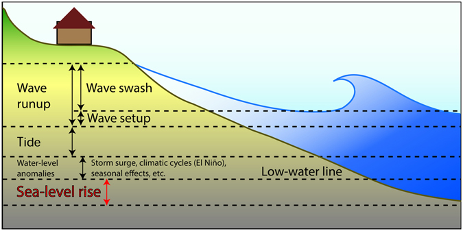
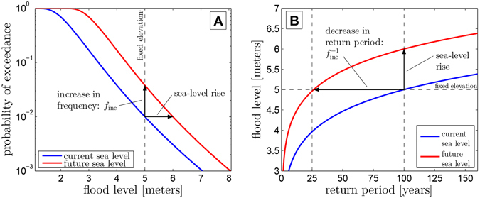
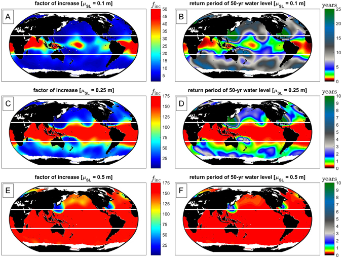
Global climate change drives sea-level rise, increasing the frequency of coastal flooding. In most coastal regions, the amount of sea-level rise occurring over years to decades is significantly smaller than normal ocean-level fluctuations caused by tides, waves, and storm surge. However, even gradual sea-level rise can rapidly increase the frequency and severity of coastal flooding. So far, global-scale estimates of increased coastal flooding due to sea-level rise have not considered elevated water levels due to waves, and thus underestimate the potential impact. Here we use extreme value theory to combine sea-level projections with wave, tide, and storm surge models to estimate increases in coastal flooding on a continuous global scale. We find that regions with limited water-level variability, i.e., short-tailed flood-level distributions, located mainly in the Tropics, will experience the largest increases in flooding frequency. The 10 to 20 cm of sea-level rise expected no later than 2050 will more than double the frequency of extreme water-level events in the Tropics, impairing the developing economies of equatorial coastal cities and the habitability of low-lying Pacific island nations.

Figure 1

The water-level components that contribute to coastal flooding.

Figure 2

Example: by elevating the exceedance probability distribution, a 1 m increase in SL increases the frequency (A) and lowers the return period (B) of the 5m-flood level. Note that the steeper the probability distribution in A, the flatter the return time curve in B, i.e., the greater the increase in frequency and the reduction in return time. Thus regions with lower variability in flood level will experience larger increases in flooding frequency under SLR. See Methods and extended data Figs 1 and 2.

Figure 3

Global estimates of the location (μ), scale (σ), and shape (k) parameters of the GEV distribution of extreme water-level (the sum of wave setup, tide, and storm surge) shown in panels A, B, and C, respectively. The dashed and solid lines in panel C represent contours of k that are significantly different from zero at the 75% and 95% confidence levels, respectively. The maps in this figure were made using Matlab 2016a (https://www.mathworks.com/products/matlab/).

Figure 4

Global estimates of the expected factor of increase in exceedance probability, f _inc, and the future return period, T _R, of the 50-yr water level, for SLR projections: μ _SL = +0.1, +0.25, +0.5 m. We note that the estimated increase in flooding potential is purely due to SLR and not due to changes in climate or storminess. White lines indicate the Tropic of Cancer and Tropic of Capricorn. The maps in this figure were made using Matlab 2016a (https://www.mathworks.com/products/matlab/).

Figure 5

The upper bound of SLR that doubles the exceedance probability of the former 50-year water level. This SLR is the upper limit of a 95% confidence interval based on a Monte Carlo simulation of the GEV parameter estimates and their associated confidence bands (see Methods). Red areas represent regions particularly vulnerable to small amounts of SLR. The maps in this figure were made using Matlab 2016a (https://www.mathworks.com/products/matlab/).

References

-
- Watson CS, et al. Unabated global mean sea-level rise over the satellite altimeter era. Nature Climate Change. 2015;5(6):565–568. doi: 10.1038/nclimate2635. - DOI
- Yi S, Sun W, Heki K, Qian A. An increase in the rate of global mean sea level rise since 2010. Geophysical Research Letters. 2015;42(10):3998–4006. doi: 10.1002/2015GL063902. - DOI
- Church, J. A. et al. Sea level change. (Climate Change 2013: The Physical Science Basis) 1137–1216. (Cambridge University Press, 2013).
- Slangen, A. B. A. et al. A review of recent updates of sea-level projections at global and regional scales. Surveys in Geophysics. (2016).
- Horton, B. P., Rahmstorf, S., Engelhart, S. E. & Kemp, A. C. Expert assessment of sea-level rise by AD 2100 and AD 2300. Quaternary Science Reviews. 84 (2014).
Publication types
LinkOut - more resources
Full Text Sources
Other Literature Sources