Reassessment of 20th century global mean sea level rise

Abstract

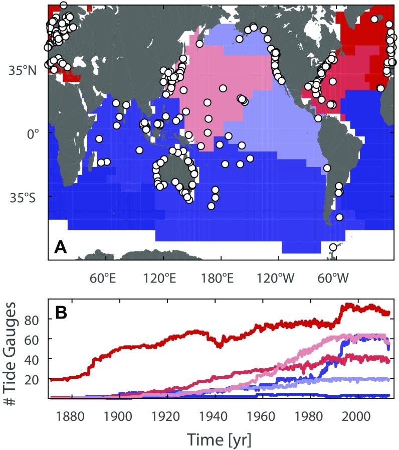
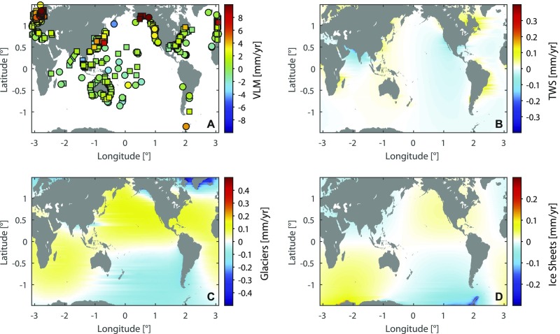
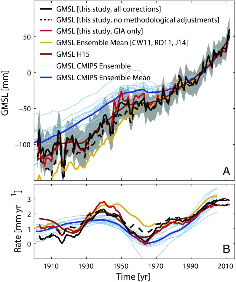
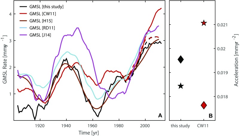
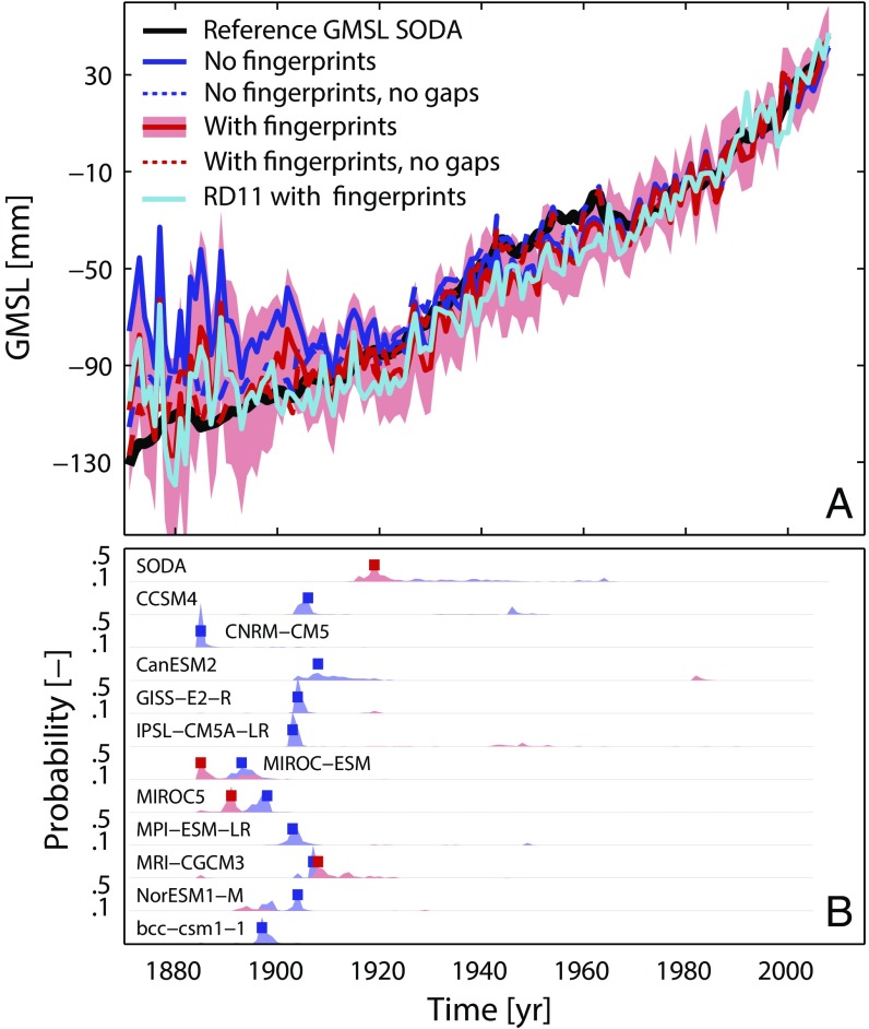
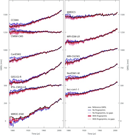
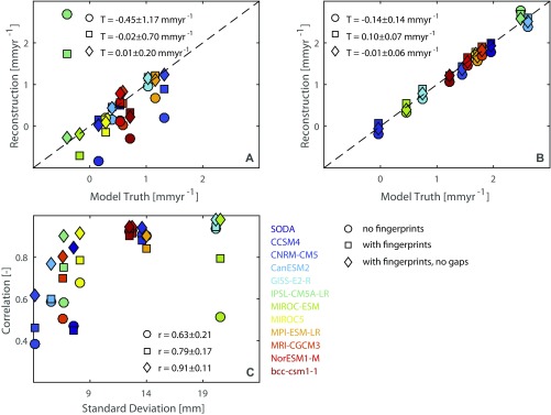
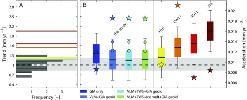
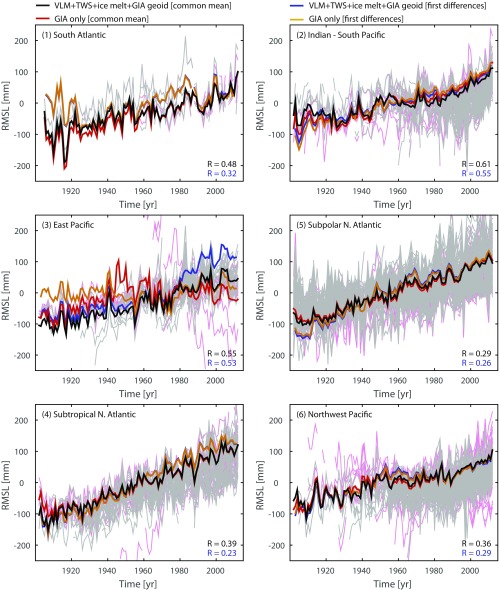
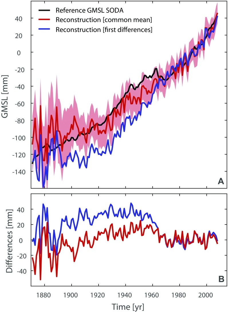
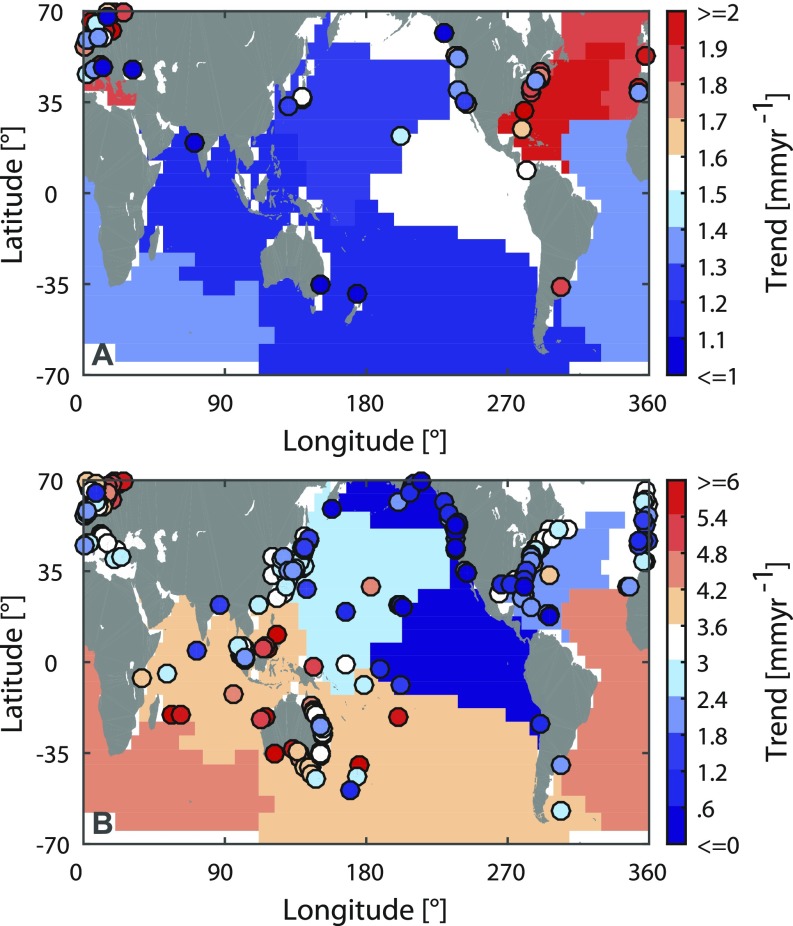
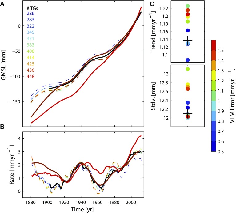
The rate at which global mean sea level (GMSL) rose during the 20th century is uncertain, with little consensus between various reconstructions that indicate rates of rise ranging from 1.3 to 2 mm⋅y^-1 Here we present a 20th-century GMSL reconstruction computed using an area-weighting technique for averaging tide gauge records that both incorporates up-to-date observations of vertical land motion (VLM) and corrections for local geoid changes resulting from ice melting and terrestrial freshwater storage and allows for the identification of possible differences compared with earlier attempts. Our reconstructed GMSL trend of 1.1 ± 0.3 mm⋅y^-1 (1σ) before 1990 falls below previous estimates, whereas our estimate of 3.1 ± 1.4 mm⋅y^-1 from 1993 to 2012 is consistent with independent estimates from satellite altimetry, leading to overall acceleration larger than previously suggested. This feature is geographically dominated by the Indian Ocean-Southern Pacific region, marking a transition from lower-than-average rates before 1990 toward unprecedented high rates in recent decades. We demonstrate that VLM corrections, area weighting, and our use of a common reference datum for tide gauges may explain the lower rates compared with earlier GMSL estimates in approximately equal proportion. The trends and multidecadal variability of our GMSL curve also compare well to the sum of individual contributions obtained from historical outputs of the Coupled Model Intercomparison Project Phase 5. This, in turn, increases our confidence in process-based projections presented in the Fifth Assessment Report of the Intergovernmental Panel on Climate Change.

Keywords: climate change; fingerprints; global mean sea level; tide gauges; vertical land motion.

Fig. S1.

Spatial and temporal availability of tide gauges used in this study. (A) Spatial distribution of the tide gauges used in this study. Also shown are the six oceanic regions, which are used to build regional virtual stations. (B) Respective temporal availability of tide gauges for each region.

Fig. S2.

Solid Earth and geoid corrections used in this study. (A) VLM [circles, GPS; square, altimetry minus tide gauge (AL-TG); diamonds, GIA] and geoid corrections resulting from (B) TWS, (C) glaciers, and (D) ice sheets.

Fig. 1.

Time series and rates of GMSL during the period 1902–2012. (A) Revised GMSL reconstruction based on 322 tide gauges in comparison with previous estimates (CW11 = ref. ; RD11 = ref. ; J14 = ref. ; H15 = ref. 6) and modeling attempts based on historical CMIP5 models (12). The gray shading marks the 1σ errors of the final reconstruction. The dotted black line represents a GMSL reconstruction with all VLM and geoid corrections, but without methodological adjustments such as area weighting and the use of a common mean. (B) The corresponding rates calculated with a singular spectrum analysis using an embedding dimension of 15 y.

Fig. S3.

Comparison of GMSL rates from tide gauges and satellite altimetry. (A) Shown are the GMSL rates from ref. (red) and our reconstruction (black), once based solely on tide gauges (solid lines), and once adjusted for GMSL from satellite altimetry (AVISO) since 1993 (dotted line). For comparison, the rates from ref. (cyan), ref. (magenta), and ref. (brown) also are shown. (B) The corresponding acceleration coefficients (diamonds, adjusted; pentagrams, original). The figure demonstrates that the ref. reconstruction overestimates GMSL since 1993 by up to 1 mm⋅y⁻¹, leading to a very large acceleration over the entire century. However, once adjusted for the “true” GMSL from AVISO satellite altimetry since 1993, the adjusted reconstructions closely follow our original reconstruction, leading to an overall acceleration that is smaller than that estimated for our original GMSL reconstruction.

Fig. 2.

Performance of the area-weighted average approach in ocean models. (A) Sensitivity of the area-weighted average technique in the SODA reanalysis (its reference GMSL is shown by the black line) to the four initial data sets: Gaps as in reality, no fingerprint corrections applied (dark blue); assuming a full record, no fingerprint corrections applied (dark blue dotted); gaps as in reality, fingerprint corrections applied (red, with shading noting its 1σ uncertainty); and assuming a full record, fingerprint corrections applied (red dotted) (Fig. S3 for the respective curves from the 11 CMIP5-based synthetic sea level fields). The cyan curve represents a GMSL reconstruction with gaps as in reality and fingerprint corrections applied, but using the tide gauge subset from ref. . (B) Results of the Bayesian change point analysis (25) on the differences between each model specific reference GMSL and corresponding tide gauge reconstruction , without fingerprint corrections; red, with fingerprint correction) in each model. The change point analysis provides statistically the probability and timing of changes (shaded areas) in the relationship between the “true” model GMSL and its reconstruction. Tall, thin spikes suggest relative certainty in the timing of a change point, whereas wider spikes suggest more uncertainty in its timing. The red and blue squares mark the most probable timing from 500 iterations.

Fig. S4.

Performance of the area-weighted average technique in synthetic sea level fields from the CMIP5 database. Comparison of reconstructed GMSL with the “true” reference GMSL in the 11 synthetic sea level fields based on CMIP5 historical simulations (dynamic sea level and glaciers) and reanalysis estimates of TWS and ice sheet melting. The sensitivity is tested for different initial data sets, as defined in the caption of Fig. 2 (showing the results for the GMSL from the SODA reanalysis).

Fig. S5.

Trend and correlation biases in GMSL reconstructions based on synthetic sea level fields from ocean models. (A) Comparison between the linear trends for the reference GMSL of each model and its reconstruction based on tide gauges with (squares) and without (circles) fingerprint corrections and assuming no gaps in tide gauge records (i.e., a fully available record; diamonds) for the period 1871–1902. (B) As A, but for the period 1902–2005. (C) Relationship between the correlation of the reference GMSL and its tide gauge reconstruction in each model and the respective interannual variability of the reference GMSL (SD). The results suggest that the GMSL can be better reconstructed in models with stronger interannual variability.

Fig. 3.

Linear trends in observed and modeled GMSL during the period 1902–1990. (A) Linear trend frequency in the CMIP5 GMSL ensemble from ref. (dark gray bars), together with the median value (thick dotted line) and the 68% confidence bounds (light gray shading). The color coding follows B. (B) Linear trends of four different GMSL realizations based on different corrections applied in comparison with previous estimates with their respective uncertainties (based on ref. 25) as boxplots (1σ and 2σ uncertainties). The dots correspond to the trends when no area weighting is applied, whereas the diamonds provide trend estimates for the reconstructions based on rate stacking without area-weighting as in ref. . Also shown is the acceleration term (pentagrams, right y axis) for each reconstruction extracted from the first differences of the nonlinear trends during the entirely available period of each reconstruction since 1902.

Fig. S6.

Virtual stations for the six oceanic regions based on different stacking approaches and corrections. Shown are the individual tide gauge records corrected for VLM, TWS, ice melting, and GIA geoid (gray) or just GIA (light red) and their respective virtual stations based on two different stacking approaches: averaging after removing a common mean, and stacking first differences (also known as rate stacking; see legend for a description of the line colors). Both approaches are used to overcome the problem of an unknown reference datum of individual tide gauges. Also provided for each region are the medians of linear correlations between the virtual stations and individual tide gauge records from both approaches (black and blue R values).

Fig. S7.

Comparison of the reference GMSL in SODA to two different reconstructions. (A) Reference GMSL (black line) and reconstructions using either a common mean between individual tide gauges (red line, shaded area gives the 1σ uncertainty) or first differences (blue curve). (B) Differences between the reference GMSL and the two reconstructions.

Fig. S8.

Trends in individual tide gauges corrected for VLM and geoid changes from TWS and ice melt. (A) Trends in tide gauges providing at least 70 y of data during the period 1902–2012. Blue colors denote trends equal or smaller than 1.5 mm⋅y⁻¹, and white and red dots mark those stations providing long-term trends above 1.5 mm⋅y⁻¹. The colored shaded areas represent the trends of the region-specific virtual stations. (B) Trends in tide gauge records providing at least 15 y of data during the period 1993–2012. Blue colors denote trends equal or smaller than 3 mm⋅y⁻¹, whereas white and red dots mark those stations providing long-term trends above 3 mm⋅y⁻¹.

Fig. S9.

Effect of tide gauge selection on GMSL and extension to 1880. (A) Shown are 11 realizations of our GMSL curve, using different subsets of tide gauges resulting from VLM error thresholds between 0.5 and 1.5 mm⋅y⁻¹, extending back to 1880 (dashed lines). Since before 1902, there is no information on the geoid corrections; these curves are corrected only for VLM. The GMSL curve from Fig. 3A, including all corrections, is shown for comparison in black. Also shown are the reconstructions from refs. and (solid red and brown lines, respectively). (B) Corresponding rates. (C) Linear trends (1902–1990) and SDs (1902–2012) from each reconstruction (colored dots) shown in A and the final curve from Fig. 3A (black cross).

References

1. Church JA, White NJ. Sea-level rise from the late 19th to the early 21st Century. Surv Geophys. 2011;32:585–602.
1. Ray RD, Douglas BC. Experiments in reconstructing twentieth-century sea levels. Prog Oceanogr. 2011;91:496–515.
1. Wenzel M, Schroeter J. Reconstruction of regional mean sea level anomalies from tide gauges using neural networks. J Geophys Res. 2010;115:C08013.
1. Calafat FM, Chambers DP, Tsimplis MN. On the ability of global sea level reconstructions to determine trends and variability. J Geophys Res. 2014;119:1572–1592.
1. Jevrejeva S, Moore JC, Grinsted A, Matthews AP, Spada G. Trends and acceleration in global and regional sea levels since 1807. Global Planet Change. 2014;113:11–22.
Publication types
LinkOut - more resources