Applying systems-level spectral imaging and analysis to reveal the organelle interactome

Abstract

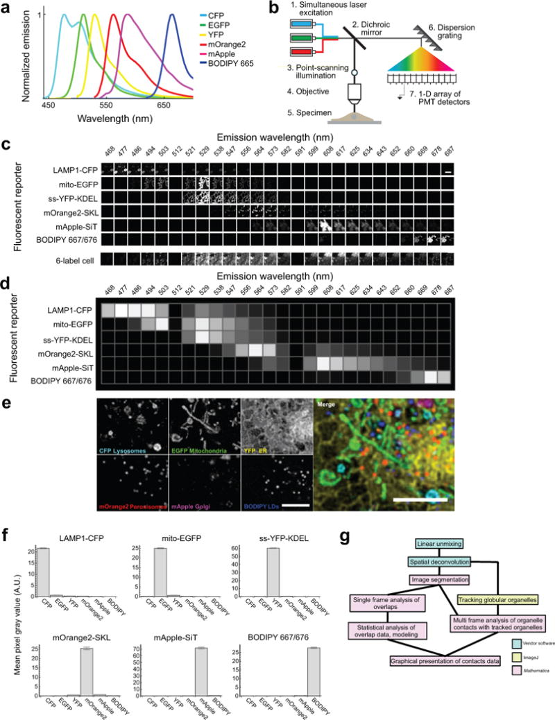
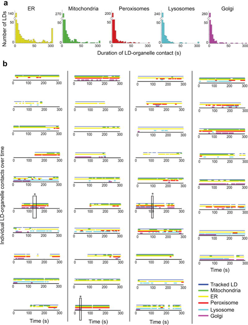
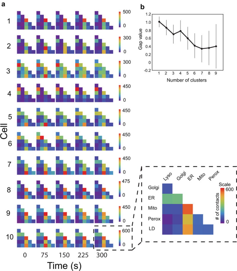
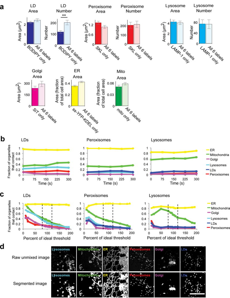
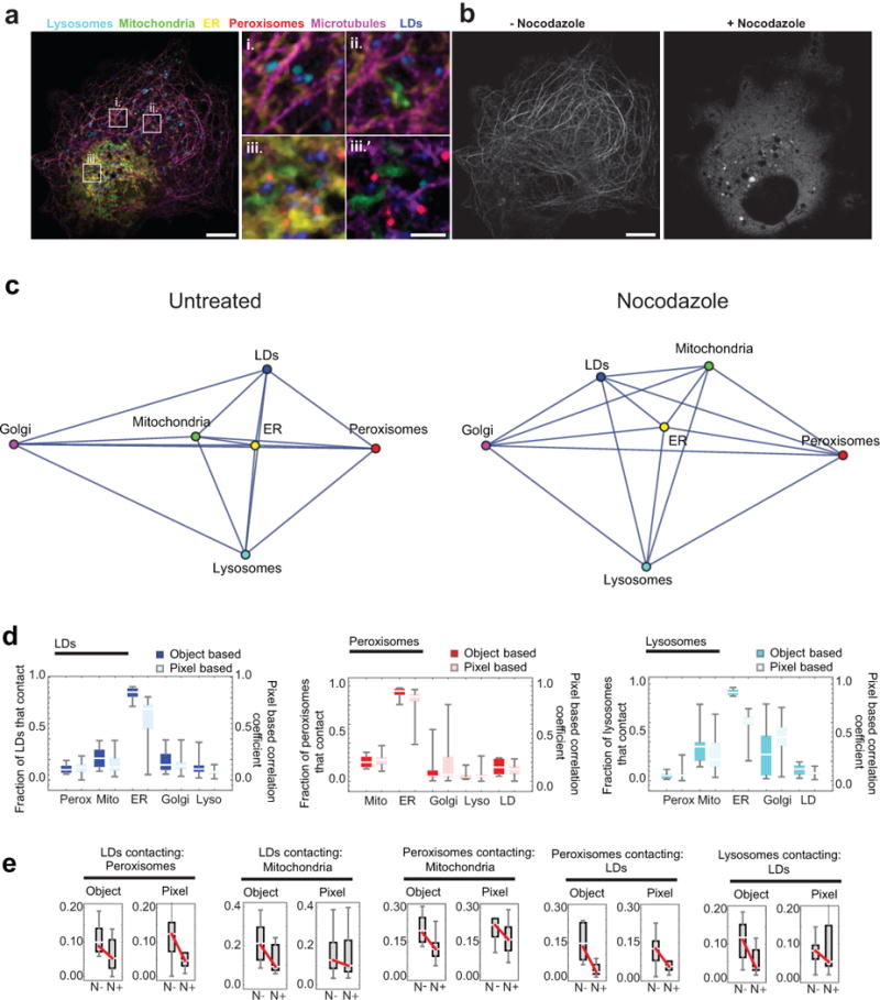
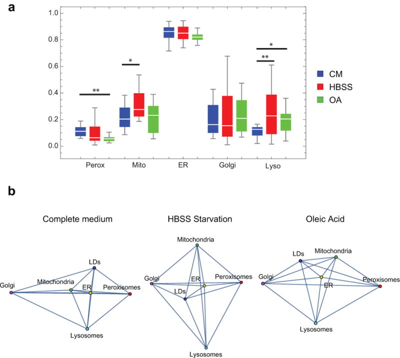
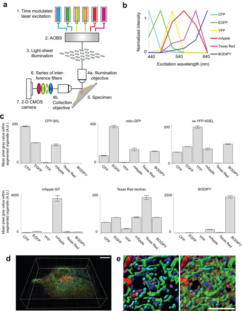
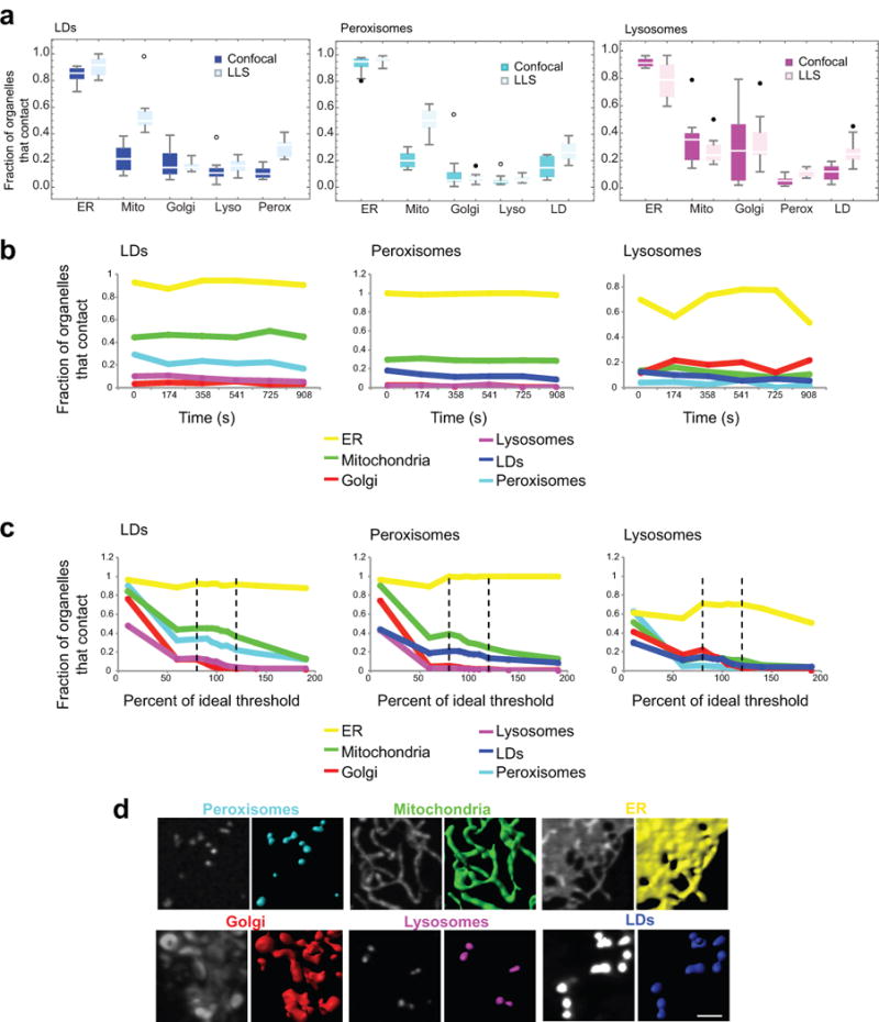
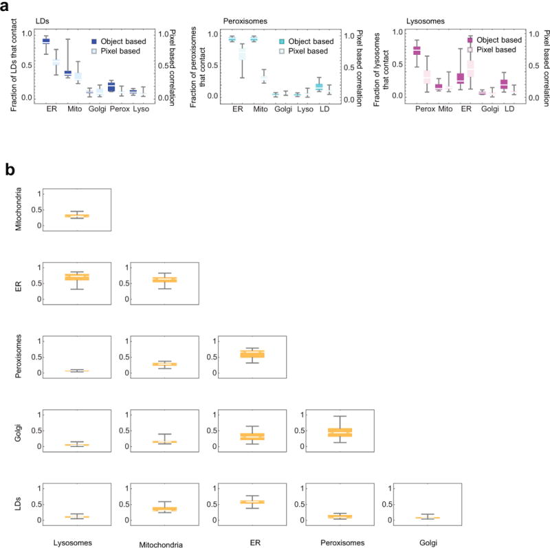
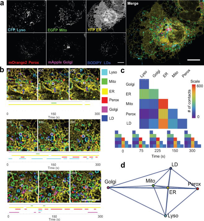
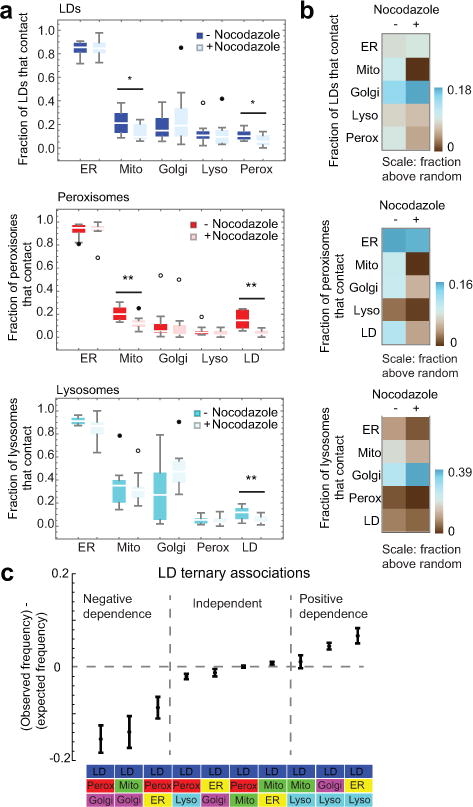
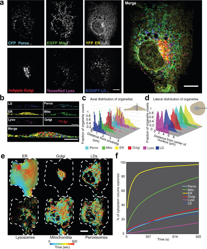
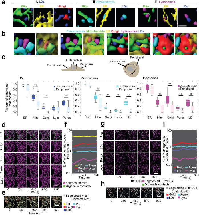
The organization of the eukaryotic cell into discrete membrane-bound organelles allows for the separation of incompatible biochemical processes, but the activities of these organelles must be coordinated. For example, lipid metabolism is distributed between the endoplasmic reticulum for lipid synthesis, lipid droplets for storage and transport, mitochondria and peroxisomes for β-oxidation, and lysosomes for lipid hydrolysis and recycling. It is increasingly recognized that organelle contacts have a vital role in diverse cellular functions. However, the spatial and temporal organization of organelles within the cell remains poorly characterized, as fluorescence imaging approaches are limited in the number of different labels that can be distinguished in a single image. Here we present a systems-level analysis of the organelle interactome using a multispectral image acquisition method that overcomes the challenge of spectral overlap in the fluorescent protein palette. We used confocal and lattice light sheet instrumentation and an imaging informatics pipeline of five steps to achieve mapping of organelle numbers, volumes, speeds, positions and dynamic inter-organelle contacts in live cells from a monkey fibroblast cell line. We describe the frequency and locality of two-, three-, four- and five-way interactions among six different membrane-bound organelles (endoplasmic reticulum, Golgi, lysosome, peroxisome, mitochondria and lipid droplet) and show how these relationships change over time. We demonstrate that each organelle has a characteristic distribution and dispersion pattern in three-dimensional space and that there is a reproducible pattern of contacts among the six organelles, that is affected by microtubule and cell nutrient status. These live-cell confocal and lattice light sheet spectral imaging approaches are applicable to any cell system expressing multiple fluorescent probes, whether in normal conditions or when cells are exposed to disturbances such as drugs, pathogens or stress. This methodology thus offers a powerful descriptive tool and can be used to develop hypotheses about cellular organization and dynamics.

Extended Data Figure 1. Strategy for 6-colour labelling, image acquisition and analysis (confocal)

Fluorescence spectral imaging has emerged as a technology that allows many different spectrally variant fluorescent markers to be distinguished in a single sample. The most widely used approach for computational analysis of spectral images, called linear unmixing (LU), involves a matrix inverse operation to find the best fit of known fluorophore spectra to that of the recorded spectrum at every pixel in a digital image. Although this and other multispectral approaches have been used in commercial instruments to distinguish multiple combinations of organic dyes in fixed microbes^, and fixed neuronal tissue, its application to multi-labelled cells and their quantitative analysis remains underdeveloped in live cell experiments. (a) Published emission spectra for the fluorophores used in confocal experiments: CFP, EGFP, YFP, mOrange2, mApple and BODIPY 665/676. (b) Schematic of the hardware used for 6-colour confocal microscopy. The specimen was excited using three lasers simultaneously, by point-scanning illumination. Emitted light was collected by a linear array of detector elements after being dispersed by a reflective dispersion grating. (c) To derive the values for the known fluorophore matrix, images of singly labelled cells were acquired at each wavelength and under the same acquisition conditions used to acquire images of 6-label cells. Intensity values centred at 512 nm and 591 nm were zero for all cells because these detector elements were blocked to prevent scattered laser excitation light from reaching the detector. (d) Graphical representation of the unmixing matrix. The normalized intensity values at each wavelength range from 0 to 1. (e) Zoom-up of a region of the cell shown in Fig. 1a. Scale bars, 5 μm. Micrographs are representative of 10 cells captured. (f) Plots of mean pixel intensity values for all 6 fluorophores in every pixel in singly labelled cells that were segmented as foreground. Cells were singly labelled with LAMP1-CFP, mito-EGFP, ss-YFP-KDEL, mOrange2-SKL, mApple-SiT, or BODIPY 665/676. n = 87,307 pixels from one cell (CFP), 5,933 pixels from one cell (EGFP), 84,127 pixels from one cell (YFP), 2,711 pixels from one cell (mOrange2), 11,804 pixels from one cell (mApple), 3,332 pixels from one cell (BODIPY 667/676). Error bars represent s.e.m. A.U. = Arbitrary Units. (g) Imaging-informatics pipeline for quantitative analysis of organelle contacts. 32-channel micrographs of samples were subjected to pixel-based LU and spatial deconvolution algorithms, resulting in 6-channel unmixed images. These images were segmented to generate features, and contacts between features (within 1 pixel, 97 nm) were analysed in single frames. Alternatively, globular organelles were tracked and their contacts with segmented features analysed over multiple frames. The pipeline is modular and involves five major components: pixel-based LU of raw image data; spatial deconvolution; segmentation of organelles to generate features; particle tracking of globular organelles over time; and integration of track data with segmented image data to identify organelle contacts between the labelled organelles. The first four modules are implemented in existing software packages, either commercially available (Zeiss Zen and Huygens software) or freely available (histogram based segmentation algorithms and TrackMate plugin in ImageJ for particle tracking)^,. For the final component of the pipeline we developed an image analysis program on the Mathematica platform (available for downloading at http://organelle-interactome.sourceforge.net) that identifies feature-based colocalization.

Extended Data Figure 2. LD-organelle contact duration and dynamics

(a) Histograms showing the duration of LD-organelle contacts in time lapse images of a single cell, acquired and analysed as described in Fig. 1b. n = 480 LD contact events from one cell. (b) All the LDs in a single cell were tracked, and their interorganelle contacts mapped with time. A blue line indicates that the LD was successfully tracked at the specified time point. Coloured lines indicate that the tracked LD was within 1 pixel (97 nm) of the following organelles at the specified time point: green, mitochondria; yellow, ER; red, peroxisome; cyan, lysosomes; magenta, Golgi. Tracks are sorted according to LD speed, from fastest to slowest. Only LDs that were tracked for at least 25 out of 60 frames are included. Boxes marked with stars indicate examples where a single LD contacts all five other organelles in the same image frame. Shown here are the contact maps for 38 randomly selected LDs from one cell.

Extended Data Figure 3. Cell-to-cell variation in the organelle interactome over time

(a) The absolute numbers of organelle contacts in each cell at a single time point are displayed as graphical half matrices. Each row in the matrix represents the number of organelle contacts with each target organelle (columns), and is colour coded from 0 to maximum number of observed contacts in each cell. Each row of graphical matrices represents the organelle interactome in one cell and each column of graphical matrices represents the organelle interactome at a specific time point (0, 75, 150, 225 or 300 s). We performed an analysis of variance (ANOVA) in order to assess the variance in organelle-organelle contacts within cells over time. The results showed that the variance between cells is significantly larger than the variance within an individual cell across time (p<1×10^−37). (b) Cluster analysis of the organelle contact data for all ten cells. The gap statistic was calculated for 1–9 hypothetical clusters (see Statistics), and no meaningful differences were found to separate the organelle associations for the ten cells. This suggested there is a reproducible and scalable pattern of organelle contacts despite cell-to-cell differences in the absolute numbers of organelles. n = 100 simulations, error bars represent s.e.m.

Extended Data Figure 4. Validation of 6-colour labelling and organelle interaction measurements (confocal)

(a) To test the effect of co-expressing all six labels on organelle properties, we compared the number and/or area of organelles in cells singly transfected with one organelle marker or incubated with BODIPY, with cells labelled with all six organelle markers. For LDs, peroxisomes, and lysosomes, mean cross-sectional area and number were measured. For Golgi, total cross-sectional area/cell was measured. For ER and mitochondria, the fraction of cell area occupied by these organelles was measured. Only LD number showed a significant difference between singly- vs. multiply-labelled conditions. n = 20 cells for all 6 labelled cells, n = 20 cells (BODIPY only), n = 14 cells (SKL only), n = 21 cells (LAMP-1 only), n = 19 cells (SiT only), n = 18 cells (ER only), n = 20 cells (mito only). ** p < 0.01 (unpaired, two-tailed t-test). Bar heights represent mean values and error bars represent s.e.m. (b) Line graphs showing the fraction of LDs, peroxisomes or lysosomes contacting each of the other labelled organelles in one cell over time, measured discreetly at 0, 75, 150, 225 and 300 s. The fraction of total LDs, peroxisomes or lysosomes contacting each of the other organelles remained constant over the course of imaging, consistent with minimal perturbation and phototoxicity during the imaging period. (c) Line graphs showing the fraction of LDs, peroxisomes or lysosomes contacting each of the other labelled organelles in one cell (cell 1 in Extended Data Fig. 3a) after modulating the threshold value for all channels by a fixed percentage. Dashed lines represent a threshold modulated up or down by 20%. Ideal threshold = 100%. For all organelles except mitochondria, modulating the threshold up or down by up to 20% from the algorithmically determined optimal threshold value did not significantly alter the measured number of organelle contacts, suggesting that our organelle contact measurements are insensitive to small differences in threshold parameters. (d) Examples of segmentation based on algorithmically-determined, optimal intensity threshold values. Micrographs are representative of 10 cells captured. Scale bar, 10 μm.

Extended Data Figure 5. Effect of nocodazole on organelle contacts

(a) Micrographs of a COS-7 cell labelled as in Fig. 1, except that instead of labelling Golgi, microtubules were labelled with mApple-MAP4-C10. i.-iii. Enlargements of the regions outlined in the left panel. iii.’ Region iii., without the ER displayed, for clarity. Lysosomes, mitochondria, the ER, peroxisomes, and LDs were all observed in close proximity to microtubules. Scale bars, 10 μm (left) and 2 μm (right). (b) The same cell as in (a), displaying only the microtubule channel, both before (left) and (after) treatment with 5 μM nocodazole for 1 h. Scale bar, 10 μm. Micrographs in (a) and (b) are representative of 20 cells captured. (c) Network diagrams of untreated and nocodazole-treated cells. Untreated network is the same as in Fig. 1d. After nocodazole treatment, the ER remains the central node in the network. (d) Comparison of object-based organelle contact analysis (bright) versus pixel-based organelle colocalization analysis (pastel). For the pixel-based analysis, a value of 1 indicates perfect co‐localization, while a value of 0 indicates the organelles are never co‐located. No statistical test was performed. (e) Comparison of the effect of nocodazole treatment on organelle contacts when images were analysed using either an object-based or pixel-based colocalization analysis scheme. Red lines connecting the median values indicate that the median number of contacts decreased after nocodazole treatment. Shown are all organelle contact pairs that showed a statistically significant change in contact frequency when cells were treated with nocodazole (unpaired, two-tailed t-test). (c-d) Object-based analysis data is the same as in Fig. 2a. n = 11 (nocodazole-treated) or n = 10 (untreated) cells from two experiments.

Extended Data Figure 6. Effect of starvation or excess fatty acids on organelle contacts

(a) Box whisker plots showing the fraction of LDs contacting each of the other labelled compartments in cells grown in complete medium (CM, blue), Hank’s balanced salt solution (HBSS, red), or complete medium supplemented with 300 μM oleic acid (OA, green) for 18 h. * 0.05 > p < 0.01, ** p < 0.01 (unpaired, two-tailed t-test). Error bars represent s.e.m. (b) Network diagrams showing the organelle interactome in cells treated as described in (a). (a-b) Complete medium data is the same as control data shown in Fig. 1d and Fig. 2a; n = 10 (complete medium), n = 15 (HBSS), or n = 14 (oleic acid) cells from two experiments.

Extended Data Figure 7. LLS spectral imaging and linear unmixing

(a) Schematic of the hardware used for 6-colour light sheet microscopy. The specimen was excited using six lasers sequentially, by LLS illumination. Emitted light passed through a series of interference filters and was collected using a sCMOS camera. (b) Plot of the emission intensity of the indicated fluorophores as a function of excitation wavelength, in images of singly labelled cells acquired as described in (a). To identify fluorophores in the image data, we applied an excitation-side unmixing algorithm (see Image Acquisition and Unmixing). Our multispectral time-lapse LLS images consisted of upwards of 7 billion sets of 6 colour-channel pixels (547 × 640 pixels per plane × 140 planes per cell × 100 time points per cell × 10 cells). Because the solution to the unmixing operation at every pixel is independent of every other pixel, we distributed the unmixing operation over 32 cores of a computer workstation. (c) Plots of mean pixel intensity values for all 6 fluorophores in every pixel in singly labelled cells that were segmented as foreground. Cells were singly labelled with CFP-SKL, mito-EGFP, ss-YFP-KDEL, mApple-SiT, Texas Red dextran, or BODIPY 665/676. The error in LLS unmixing is higher than for confocal (see Extended Data Fig. 1f) as expected and is due partly to the fact that only six channels of spectral information were used to unmix the overlapping spectra. n = 149 pixels (CFP), n = 3,910 pixels (EGFP), n = 9,180 pixels (YFP), n = 1,549 pixels (mApple), n = 806 pixels (Texas Red Dextran), n = 3,248 pixels (BODIPY 667/676). Error bars represent s.e.m. (d) Tilted volume rendering of the same cell shown in Fig. 3a. Scale bar, 10 μm. (e) Zoomed, segmented images from the cell shown in (d). The left panel does not include the ER channel while the right panel does (transparent yellow). Scale bar, 5 μm. Micrographs in (d) and (e) are representative of 10 cells captured.

Extended Data Figure 8. Validation of organelle interaction measurements (LLS)

(a) Box whisker plots showing the median fraction of LDs, peroxisomes, or lysosomes making contact with each of the other labelled compartments in data obtained using confocal (bright) or LLS (pastel) microscopy. Confocal data is the same as in Fig. 2a. n = 10 cells (confocal), n = 10 cells (LLS). No statistical test was performed. The similarity in measurements from LLS and confocal images is likely because the globular organelles that we examined are smaller than the depth of focus of the confocal microscope, ensuring that all their inter-organelle interactions were detected even in the confocal images. (b) Line graphs showing the fraction of LDs, peroxisomes or lysosomes contacting each of the other labelled organelles in one cell measured over time at discreet points: 0, 174, 358, 541, 725 and 908 s. (c) Line graphs showing the fraction of LDs, peroxisomes or lysosomes contacting each of the other labelled organelles in one cell after modulating the threshold value for all channels by a fixed percentage. Dashed lines represent a threshold modulated by 20%. (d) Examples of segmentation performed using the ideal threshold (i.e., 100%) in (c). Scale bar, 2 μm. Micrographs are representative of 10 cells.

Extended Data Figure 9. Comparison of object- versus pixel-based analysis (LLS)

(a) Comparison of object-based organelle contact analysis (bright) versus pixel-based organelle colocalization analysis (pastel). Object-based analysis data is the same as LLS data in Extended Data Fig. 8a. For the pixel-based analysis, a value of 1 indicates perfect co‐localization, a value of 0 indicates the organelles are never co‐located. No statistical test was performed. (b) Half matrix showing pixel-based colocalization analysis for all the labelled organelle pairs, including those that were not included in the object-based analysis. Outliers were not identified. (a-b) n = 10 cells.

Figure 1. Live-cell, 6-colour confocal microscopy to characterize the organelle interactome

(a) Micrographs of a COS-7 cell expressing LAMP1-CFP, mito-EGFP, ss-YFP-KDEL, mOrange2-SKL, and mApple-SiT, and labelled with BODIPY 665/676. Micrographs are representative of 10 cells captured. (b) LDs (outlined in white) were tracked, and their interorganelle contacts mapped. A blue line indicates that the LD was successfully tracked, while coloured lines indicate that the LD was within 1 pixel (97 nm) of the indicated organelle at the specified time point. Numbers on the micrographs represent time (s). For more examples, see Extended Data Fig. 2. (c) Top: Matrix representation of the organelle interactome. The absolute numbers of organelle contacts in a single cell at a single time point are displayed as a graphical half matrix. Each row in the matrix represents the number of organelle contacts with each target organelle (columns), and is colour coded from 0 to 600. Bottom: Organelle interactome over time. Each half matrix represents the organelle interactome in a single cell at a specific time point. (d) Network representation of the organelle interactome in all ten cells. All nodes (organelles) are connected and the length of the edges connecting two nodes represents the inverse of the number of contacts between those two organelles. Mito, mitochondria; perox, peroxisomes; lyso, lysosomes. Scale bars, (a) 10 μm, (b) 5 μm.

Figure 2. The organelle interactome depends on an intact microtubule cytoskeleton

(a) Box whisker plots showing the median fraction of LDs, peroxisomes or lysosomes contacting each of the other labelled compartments in control (-Nocodazole) or nocodazole-treated (+Nocodazole) COS-7 cells. While the total number of contacts between two populations of organelles was, by definition, the same, the fractions of each of the populations in contact were not always symmetric because some individual organelles made simultaneous contact with two or more organelles of the same type. (b) Heat map comparison of control and nocodazole-treated cells to computer models of cells with random organelle distributions. The mean values for each interaction were calculated, then the mean value for random associations was subtracted, to give the frequency of associations above random for each binary organelle interaction in the absence or presence of nocodazole. (a-b) n = 11 (nocodazole-treated) or n = 10 (untreated) cells from two experiments. * 0.05 > p < 0.01, ** p < 0.01 (unpaired two-tailed t-test). (c) Plot of observed LD ternary contact frequency minus expected frequency, assuming the probabilities of all contacts are independent of each other. n = 10 cells. Error bars represent standard error of the mean (s.e.m).

Figure 3. Live-cell, 6-colour 4D LLS microscopy to characterize organelle distribution in space and time

(a) Maximum intensity projections of a COS-7 cell expressing CFP-SKL, mito-EGFP, ss-YFP-KDEL, and mApple-SiT, and labelled with Texas Red dextran and BODIPY 665/676. (b) XZ images of segmented LLS images. (c-d) Distributions of organelles in the axial (c) and lateral (d) dimensions of a single COS-7 cell, representative of 10 cells captured. (e) Organelle dispersion in the cell over time. Voxels are colour coded according to the time that an organelle last occupied that voxel. Shown are 2-D projections where only the outer shell of the volume is visible. Cell was masked using the total dispersion of the ER as a proxy for the cell boundary. Dashed white lines represent the 2-D projected outline of the cell generated from the mask. See Video 5 to explore the volume in depth. (f) Dispersion analysis. The summed fractional cytoplasmic volume (excluding the nucleus) occupied by each organelle is plotted as a function of time. Scale bars, (a, e) 10 μm, (b) 5 μm. Micrographs are representative of 10 cells.

Figure 4. LLS analysis of the organelle interactome in 3D

(a) Examples of LD- (i.), peroxisome- (ii.) and lysosome- (iii.) interorganelle contacts in segmented LLS images. For clarity, only two channels are shown. (b) Examples of complex interorganelle contacts and organisation in segmented LLS images. (i.-iv.) The ER (transparent yellow) is shown in the right panels only. (c) Box whisker plots showing the median fraction of LDs, peroxisomes, or lysosomes contacting each of the other labelled compartments in the juxtanuclear or peripheral regions of the cell. n = 10 cells. ** p < 0.01 (paired two-tailed t-test). (d) Fields of view from volume rendered images of mitochondria (magenta) and sites of mitochondrial contact with five other organelles (green) in LLS images at discreet time points. (e) Fields of view from volume rendered images of mitochondria (grey) and sites of mitochondrial contact with all five other organelles. (f) Percentage of segmented mitochondria voxels that contact other organelles over time in the cell shown in (d-e). (g) Fields of view from volume rendered images of ERMCSs (magenta) and sites of contact with four other organelles (green). (h) Fields of view from volume rendered images of ERMCSs (grey) and sites of contact with all five other organelles. (i) Percentage of ERMCS voxels that contact other organelles over time in the cell shown in (g-h). Scale bars: (a-b) 2 μm, (d-e, g-h) 5 μm. Micrographs are representative of 10 cells captured.

References

1. Barbosa AD, Savage DB, Siniossoglou S. Lipid droplet–organelle interactions: emerging roles in lipid metabolism. Curr Opin Cell Biol. 2015;35:91–97. - PubMed
1. Shai N, Schuldiner M, Zalckvar E. No peroxisome is an island - Peroxisome contact sites. Biochim Biophys Acta. 2015 doi: 10.1016/j.bbamcr.2015.09.016. - DOI - PMC - PubMed
1. Settembre C, Fraldi A, Medina DL, Ballabio A. Signals from the lysosome: a control centre for cellular clearance and energy metabolism. Nat Rev Mol Cell Biol. 2013;14:283–296. - PMC - PubMed
1. Tatsuta T, Scharwey M, Langer T. Mitochondrial lipid trafficking. Trends Cell Biol. 2014;24:44–52. - PubMed
1. Phillips MJ, Voeltz GK. Structure and function of ER membrane contact sites with other organelles. Nat Rev Mol Cell Biol. 2016;17:69–82. - PMC - PubMed
Extended Data References
1. Garini Y, Young IT, McNamara G. Spectral imaging: Principles and applications. Cytometry A. 2006;69A:735–747. - PubMed
1. Valm AM, et al. Systems-level analysis of microbial community organization through combinatorial labeling and spectral imaging. Proc Natl Acad Sci U S A. 2011;108:4152–4157. - PMC - PubMed
1. Valm AM, Oldenbourg R, Borisy GG. Multiplexed Spectral Imaging of 120 Different Fluorescent Labels. PloS One. 2016;11:e0158495. - PMC - PubMed
1. Tsuriel S, Gudes S, Draft RW, Binshtok AM, Lichtman JW. Multispectral labeling technique to map many neighboring axonal projections in the same tissue. Nat Methods. 2015;12:547–552. - PubMed
1. Shaner NC, Steinbach PA, Tsien RY. A guide to choosing fluorescent proteins. Nat Methods. 2005;2:905–909. - PubMed
Publication types