Compensatory and decompensatory alterations in cardiomyocyte Ca2+ dynamics in hearts with diastolic dysfunction following aortic banding

Abstract

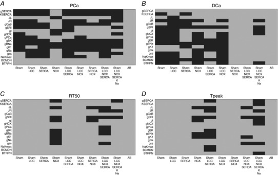
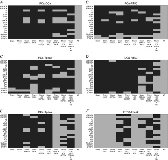
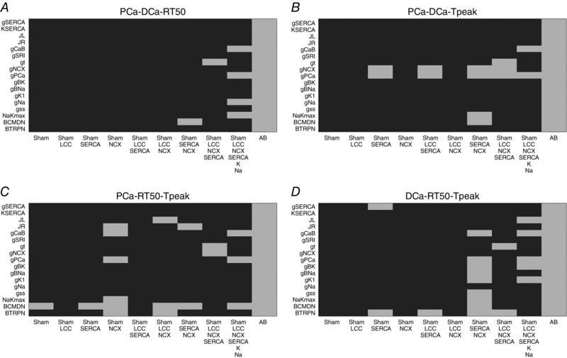
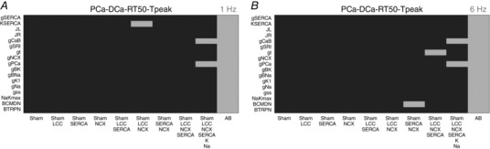
Key points: At the cellular level cardiac hypertrophy causes remodelling, leading to changes in ionic channel, pump and exchanger densities and kinetics. Previous studies have focused on quantifying changes in channels, pumps and exchangers without quantitatively linking these changes with emergent cellular scale functionality. Two biophysical cardiac cell models were created, parameterized and validated and are able to simulate electrophysiology and calcium dynamics in myocytes from control sham operated rats and aortic-banded rats exhibiting diastolic dysfunction. The contribution of each ionic pathway to the calcium kinetics was calculated, identifying the L-type Ca²⁺ channel and sarco/endoplasmic reticulum Ca²⁺ ATPase as the principal regulators of systolic and diastolic Ca²⁺ , respectively. Results show that the ability to dynamically change systolic Ca²⁺ , through changes in expression of key Ca²⁺ modelling protein densities, is drastically reduced following the aortic banding procedure; however the cells are able to compensate Ca²⁺ homeostasis in an efficient way to minimize systolic dysfunction.

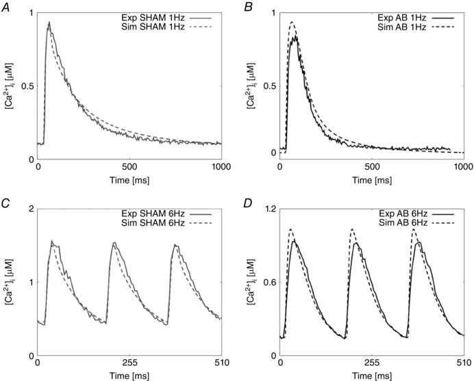
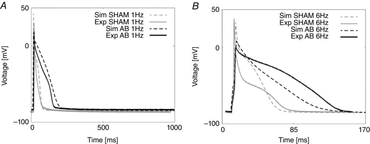
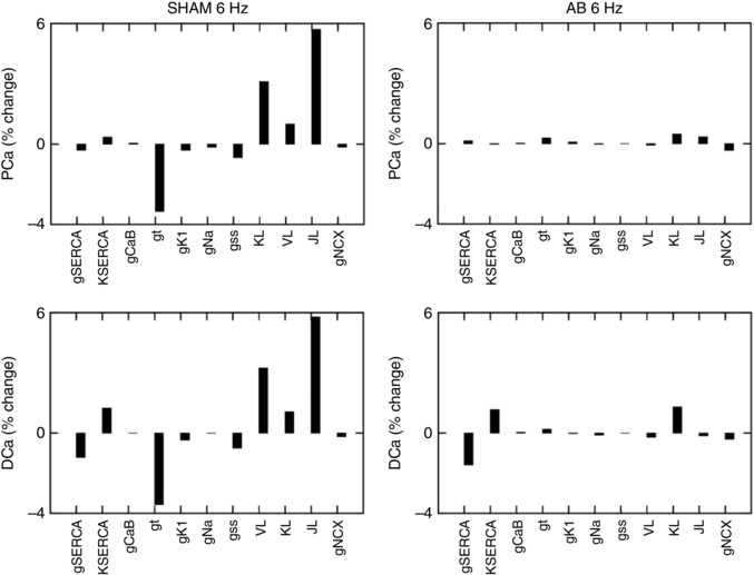
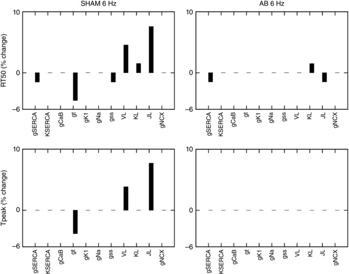
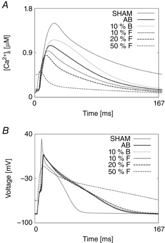
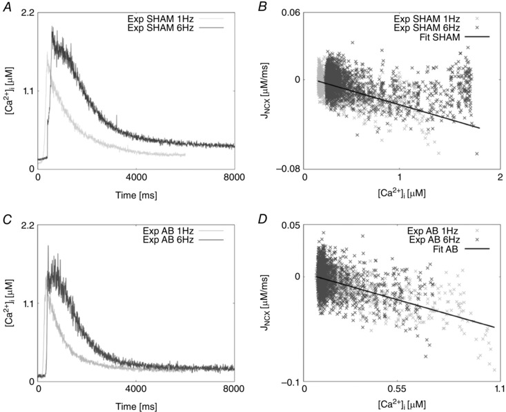
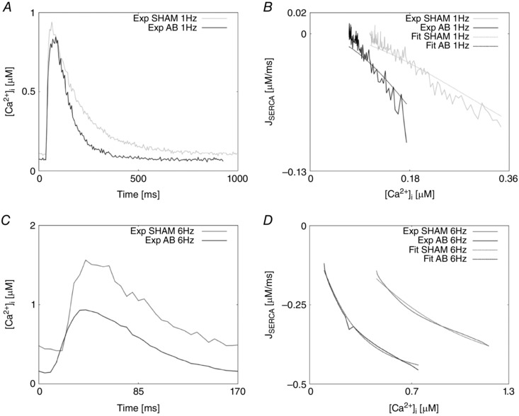
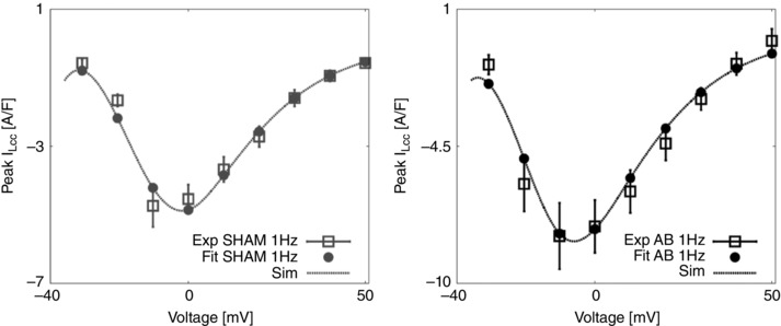
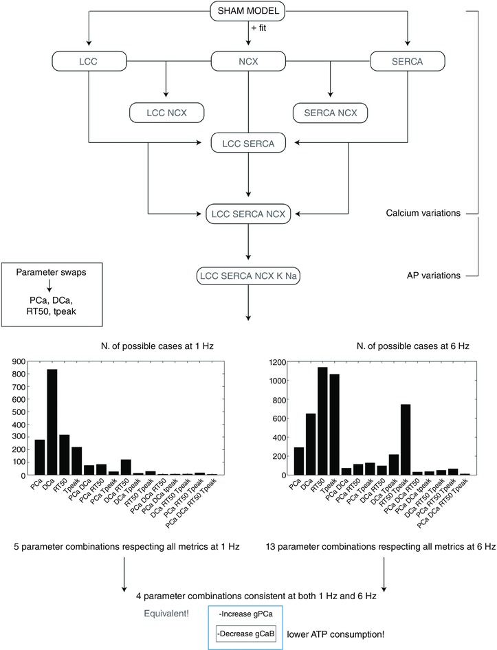
Abstract: Elevated left ventricular afterload leads to myocardial hypertrophy, diastolic dysfunction, cellular remodelling and compromised calcium dynamics. At the cellular scale this remodelling of the ionic channels, pumps and exchangers gives rise to changes in the Ca²⁺ transient. However, the relative roles of the underlying subcellular processes and the positive or negative impact of each remodelling mechanism are not fully understood. Biophysical cardiac cell models were created to simulate electrophysiology and calcium dynamics in myocytes from control rats (SHAM) and aortic-banded rats exhibiting diastolic dysfunction. The model parameters and framework were validated and the fitted parameters demonstrated to be unique for explaining our experimental data. The contribution of each ionic pathway to the calcium kinetics was calculated, identifying the L-type Ca²⁺ channel (LCC) and the sarco/endoplasmic reticulum Ca²⁺ -ATPase (SERCA) as the principal regulators of systolic and diastolic Ca²⁺ , respectively. In the aortic banding model, the sensitivity of systolic Ca²⁺ to LCC density and diastolic Ca²⁺ to SERCA density decreased by 16-fold and increased by 23%, respectively, relative to the SHAM model. The energy cost of ionic homeostasis is maintained across the two models. The models predict that changes in ionic pathway densities in compensated aortic banding rats maintain Ca²⁺ function and efficiency. The ability to dynamically alter systolic function is significantly diminished, while the capacity to maintain diastolic Ca²⁺ is moderately increased.

Keywords: calcium dynamics; cardiac electrophysiology; cell biology; computational modelling; diastolic dysfunction; gene expression; hypertrophy; rat.

Figure 1. Calcium fitting results

A, experimental representative Ca²⁺ transient for the SHAM case at 1 Hz (continuous grey line) and Ca²⁺ fitted transient (dashed grey line). B, experimental representative Ca²⁺ transient for the AB case at 1 Hz (continuous black line) and Ca²⁺ fitted transient (dashed black line). C, experimental representative Ca²⁺ transient for the SHAM case at 6 Hz (continuous grey line) and Ca²⁺ fitted transient (dashed grey line). D, experimental representative Ca²⁺ transient for the AB case at 6 Hz (continuous black line) and Ca²⁺ fitted transient (dashed black line).

Figure 2. AP fitting results

A, experimental and simulated AP traces for the SHAM case (grey) and the AB case (black) at 1 Hz. B, experimental and simulated AP traces for the SHAM case (grey) and the AB case (black) at 6 Hz.

Figure 3. Sensitivity analysis on PCa and DCa at 1%

Percentage changes in peak [Ca²⁺]i (PCa) and diastolic [Ca²⁺]i (DCa) in the SHAM case (left panels) and AB case (right panels). Sensitivity was studied by performing a 1% increase of the most important protein parameters changing from SHAM to AB: g _SERCA, K _SERCA, g _CaB, g _t, g _K1, g _Na, g _ss, J _L and g _NCX. In the case of the sensitivity value being positive, an increase in the parameter will lead to an increase in the output. In the case of the sensitivity value being negative, an increase in the parameter will lead to a decrease in the output.

Figure 4. Sensitivity analysis on RT₅₀ and T _peak at 1%

Percentage change in relaxation time at 50% (RT₅₀) and time to peak [Ca²⁺]_i (T _PEAK) in the SHAM case (left panels) and AB case (right panels). Sensitivity was studied by performing a 1% increase of the most important protein parameters changing from SHAM to AB: g _SERCA, K _SERCA, g _CaB, g _t, g _K1, g _Na, g _ss, J _L and g _NCX. In the case of the sensitivity value being positive, an increase in the parameter will lead to an increase in the output. In the case of the sensitivity value being negative, an increase in the parameter will lead to a decrease in the output.

Figure 5. Backward and forward projections

Starting from the AB model, we performed a 10% backward change in all parameters (towards the SHAM case) and a 10%, 20% and 50% forward change in all parameters (towards the AB case). A, simulated changes in the calcium transient. B, simulated changes in the AP.

Figure 6. Caffeine transients and NCX fitting results

A, experimentally measured caffeine‐induced transients for the SHAM case recorded at 1 Hz (light grey) and 6 Hz (dark grey). B, NCX flux (J _NCX) as a function of internal Ca²⁺ in the SHAM case at 1 Hz (light grey) and 6 Hz (dark grey). The fitting is represented by a straight line (black). C, experimentally measured caffeine‐induced transients for the AB case recorded at 1 Hz (light grey) and 6 Hz (dark grey). D, NCX flux (J _NCX) as a function of internal Ca²⁺ in the AB case at 1 Hz (light grey) and 6 Hz (dark grey). The fitting is represented by a straight line (black).

Figure 7. Calcium transients and SERCA fitting results

A, experimentally measured Ca²⁺ transients recorded at 1 Hz in the SHAM case (grey) and AB case (black). B, SERCA flux (J _SERCA) as a function of internal Ca²⁺ at 1 Hz in the SHAM case (continuous grey line) and AB case (continuous black line). Fittings at 1 Hz are represented in the SHAM case (dashed grey line) and AB case (dashed black line). C, experimentally measured Ca²⁺ transients recorded at 6 Hz in the SHAM case (grey) and AB case (black). D, SERCA flux (J _SERCA) as a function of internal Ca²⁺ at 6 Hz in the SHAM case (continuous grey line) and AB case (continuous black line). Fittings at 6 Hz are represented in the SHAM case (dashed grey line) and AB case (dashed black line).

Figure 8. LCC fitting procedure and results

Left, bell shaped peak I _LCC–V relationship, experiments for the SHAM case at 1 Hz are represented as mean ± standard deviation (grey boxes) and fit (grey circles and dashed grey line). Right, bell shaped peak I _LCC–V relationship, experiments for the AB case at 1 Hz are represented as mean ± standard deviation (black boxes) and fit (black circles and dashed black line).

Figure 9. Schematic representation of the validation method

Starting from the SHAM model at 1 Hz we have developed nine models by introducing single fittings for LCC, SERCA and NCX (3 models), combination of those (4 models) and all the fittings plus changes in K⁺ and Na⁺ channels (1 model) and K⁺, Na⁺ and CaB channels (1 model). For each of the nine models we have then performed parameter swaps of the most important protein parameters: g _SERCA, K _SERCA, J _L, J _R, g _CaB, g _SRl, g _t, g _NCX, g _pCa, g _BK, g _BNa, g _K1, g _Na, g _ss, NaK_max, B _CMDN and B _TRPN. The same process was repeated at 6 Hz. All developed models, representing 5814 parameter combinations (18 models × 17 parameters × 19 values) were run to steady state. For each model we have recorded PCa, DCa, RT₅₀ and T _peak. Ultimately, we have observed the number of combinations for which simulated PCa, DCa, RT₅₀ and DCa fall within 20% variability of those four experimentally measured metrics. [Color figure can be viewed at wileyonlinelibrary.com]

Figure 10. Single metrics at 1 Hz

Parameters combinations falling inside (grey) and outside (black) single metrics experimental ranges. A, possible combinations of parameters falling inside a 20% variability range from PCa experimental measurements (grey). B, possible combinations of parameters falling inside a 20% variability range from DCa experimental measurements (grey). C, possible combinations of parameters falling inside a 20% variability range from RT₅₀ experimental measurements (grey). D, possible combinations of parameters falling inside a 20% variability range from T _peak experimental measurements (grey).

Figure 11. Metric couples at 1 Hz

Parameters combinations falling inside (grey) and outside (black) experimental ranges for two metrics. A, possible combinations of parameters falling inside a 20% variability range from PCa and DCa experimental measurements (grey). B, possible combinations of parameters falling inside a 20% variability range from PCa and RT₅₀ experimental measurements (grey). C, possible combinations of parameters falling inside a 20% variability range from PCa and T _peak experimental measurements (grey). D, possible combinations of parameters falling inside a 20% variability range from DCa and RT₅₀ experimental measurements (grey). E, possible combinations of parameters falling inside a 20% variability range from DCa and T _peak experimental measurements (grey). F, possible combinations of parameters falling inside a 20% variability range from RT₅₀ and T experimental measurements (grey).

Figure 12. Metric triplets at 1 Hz

Parameters combinations falling inside (grey) and outside (black) experimental ranges for three metrics. A, possible combinations of parameters falling inside a 20% variability range from PCa, DCa and RT₅₀ experimental measurements (grey). B, possible combinations of parameters falling inside a 20% variability range from PCa DCa and T _peak experimental measurements (grey). C, possible combinations of parameters falling inside a 20% variability range from PCa, RT₅₀ and T _peak experimental measurements (grey). D, possible combinations of parameters falling inside a 20% variability range from DCa, RT₅₀ and T _peak experimental measurements (grey).

Figure 13. Single metrics at 6 Hz

Parameters combinations falling inside (grey) and outside (black) single metrics experimental ranges. A, possible combinations of parameters falling inside a 20% variability range from PCa experimental measurements (grey). B, possible combinations of parameters falling inside a 20% variability range from DCa experimental measurements (grey). C, possible combinations of parameters falling inside a 20% variability range from RT₅₀ experimental measurements (grey). D, possible combinations of parameters falling inside a 20% variability range from T _peak experimental measurements (grey).

Figure 14. Metric couples at 6 Hz

Parameters combinations falling inside (grey) and outside (black) experimental ranges for two metrics. A, possible combinations of parameters falling inside a 20% variability range from PCa and DCa experimental measurements (grey). B, possible combinations of parameters falling inside a 20% variability range from PCa and RT₅₀ experimental measurements (grey). C, possible combinations of parameters falling inside a 20% variability range from PCa and T _peak experimental measurements (grey). D, possible combinations of parameters falling inside a 20% variability range from DCa and RT₅₀ experimental measurements (grey). E, possible combinations of parameters falling inside a 20% variability range from DCa and T _peak experimental measurements (grey). F, possible combinations of parameters falling inside a 20% variability range from RT₅₀ and T _peak experimental measurements (grey).

Figure 15. Metric triplets at 6 Hz

Parameters combinations falling inside (grey) and outside (black) experimental ranges for three metrics. A, possible combinations of parameters falling inside a 20% variability range from PCa, DCa and RT₅₀ experimental measurements (grey). B, possible combinations of parameters falling inside a 20% variability range from PCa DCa and T _peak experimental measurements (grey). C, possible combinations of parameters falling inside a 20% variability range from PCa, RT₅₀ and T _peak experimental measurements (grey). D, possible combinations of parameters falling inside a 20% variability range from DCa, RT₅₀ and T _peak experimental measurements (grey).

Figure 16. All metrics at 6 Hz

Parameters combinations falling inside (grey) and outside (black) all metrics experimental ranges. A, possible combinations of parameters falling inside a 20% variability range from PCa, DCa, RT₅₀ and T _peak experimental measurements at 1 Hz (grey). B, possible combinations of parameters falling inside a 20% variability range from PCa, DCa, RT₅₀ and T _peak experimental measurements at 6 Hz (grey).

References

1. Aeschbacher BC, Hutter D, Fuhrer J, Weidmann P, Delacrétaz E & Allemann Y (2001). Diastolic dysfunction precedes myocardial hypertrophy in the development of hypertension. Am J Hypertens 14, 106–113. - PubMed
1. Amin AS, Tan HL & Wilde AAM (2010). Cardiac ion channels in health and disease. Hear Rhythm 7, 117–126. - PubMed
1. Bailey BA & Houser SR (1992). Calcium transients in feline left ventricular myocytes with hypertrophy induced by slow progressive pressure overload. J Mol Cell Cardiol 24, 365–373. - PubMed
1. Balke CW & Shorofsky SR (1998). Alterations in calcium handling in cardiac hypertrophy and heart failure. Cardiovasc Res 37, 290–299. - PubMed
1. Bénitah JP, Gomez AM, Bailly P, Da Ponte JP, Berson G, Delgado C & Lorente P (1993). Heterogeneity of the early outward current in ventricular cells isolated from normal and hypertrophied rat hearts. J Physiol 469, 111–138. - PMC - PubMed
Publication types