. 2017 Aug:137:1-23.
doi: 10.1016/j.visres.2017.05.003. Epub 2017 Jul 12.

Two representations of a high-dimensional perceptual space

Affiliations

Two representations of a high-dimensional perceptual space

Jonathan D Victor et al. Vision Res. 2017 Aug.

Abstract

A perceptual space is a mental workspace of points in a sensory domain that supports similarity and difference judgments and enables further processing such as classification and naming. Perceptual spaces are present across sensory modalities; examples include colors, faces, auditory textures, and odors. Color is perhaps the best-studied perceptual space, but it is atypical in two respects. First, the dimensions of color space are directly linked to the three cone absorption spectra, but the dimensions of generic perceptual spaces are not as readily traceable to single-neuron properties. Second, generic perceptual spaces have more than three dimensions. This is important because representing each distinguishable point in a high-dimensional space by a separate neuron or population is unwieldy; combinatorial strategies may be needed to overcome this hurdle. To study the representation of a complex perceptual space, we focused on a well-characterized 10-dimensional domain of visual textures. Within this domain, we determine perceptual distances in a threshold task (segmentation) and a suprathreshold task (border salience comparison). In N=4 human observers, we find both quantitative and qualitative differences between these sets of measurements. Quantitatively, observers' segmentation thresholds were inconsistent with their uncertainty determined from border salience comparisons. Qualitatively, segmentation thresholds suggested that distances are determined by a coordinate representation with Euclidean geometry. Border salience comparisons, in contrast, indicated a global curvature of the space, and that distances are determined by activity patterns across broadly tuned elements. Thus, our results indicate two representations of this perceptual space, and suggest that they use differing combinatorial strategies.

Significance statement: To move from sensory signals to decisions and actions, the brain carries out a sequence of transformations. An important stage in this process is the construction of a "perceptual space" - an internal workspace of sensory information that captures similarities and differences, and enables further processing, such as classification and naming. Perceptual spaces for color, faces, visual and haptic textures and shapes, sounds, and odors (among others) are known to exist. How such spaces are represented is at present unknown. Here, using visual textures as a model, we investigate this. Psychophysical measurements suggest roles for two combinatorial strategies: one based on projections onto coordinate-like axes, and one based on patterns of activity across broadly tuned elements scattered throughout the space.

Keywords: Border salience; Intermediate vision; Local features; Multipoint correlations; Visual textures.


Figures

Figure 1
Figure 1
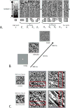
The space of visual textures, and the segmentation task for measuring thresholds. Panel A shows the 10 coordinates of the space. Γ is the difference between the fraction of white checks and the fraction of black checks; the other coordinates (the β’s, the θ’s, and α) quantify correlations among two, three, and four checks within a 2 × 2 neighborhood. The strips show the effects of varying each coordinate through its allowable range (−1 to +1); the origin of the space (all coordinates equal to 0) is the random texture. Panel B shows the stimulus sequence for the segmentation task: a fixation spot, followed by a 64 × 64 array of checks containing an embedded 16 × 64 -check target, followed by a mask. C: Stimulus examples. Top row, left: the reference texture is random, the target has a value of β\ = 0.6; right: background and target textures are interchanged. Bottom row, left: the reference texture has (β\, β/) = (0.35,0.35); the target has values (β\, β/) = (0.95,0.35); right: background and target textures are interchanged. Red contour indicating target is for illustrative purposes and was not present in the experimental stimuli. Panel A adapted from Figure 1 of (Victor et al., 2015), with permission of the copyright holder, Elsevier B.V. Panel B adapted from Figure 1 of (Victor et al., 2013), with permission of the copyright holder, The Association for Research in Vision and Ophthalmology.
Figure 2
Figure 2
The border salience task. Panel A: The (β\, β/) -plane of visual textures, illustrating selection of five test points {x2,x1,x0,x1,x2} (designated x−2, …, x2 in the Figure). B. Four example stimuli. Each stimulus is divided into four quadrants. The textures displayed in each quadrant are determined by a random choice of three test points; one of the test points is used for two adjacent quadrants. The choice of test points is indicated below each example; the point labels indicate their locations in Panel A. Black arrows indicate texture borders; the white arrows indicate the null border between two quadrants determined by the same test point.
Figure 3
Figure 3
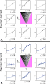
Thresholds for texture segmentation around the origin (panel A) and around the reference point (γ, β_) = (0,0.6) (panel B). Each plot shows psychometric functions for the segmentation task in eight directions in the (γ, β_) -plane; the central panel shows the stimulus domain for (γ, β_). The labels under each plot indicate the maximum displacement from the reference point. Smooth curves are Weibull function fits with a common value of the shape parameter br for all rays (eq. (1)); error bars are 95% confidence intervals. Subject: MC.
Figure 4
Figure 4
A. The (γ, β_) stimulus domain. B. Isodiscrimination contours around the origin (gray) and four peripheral reference points within the (γ, β_) plane (colors). Peripheral reference points were at (γ, β_) = {(±0.3,0), (0,±0.6)}. C. Characteristic distance to threshold at the origin and at four peripheral reference points, determined by the radius of the circle whose area equals the area of the isodiscrimination contour. Colors correspond to the isodiscrimination contours in A. Error bars: 95% confidence intervals. Four subjects.
Figure 5
Figure 5
A. The (β_, β|) stimulus domain. B. Isodiscrimination contours around the origin (gray) and eight peripheral reference points within the (β_, β|) plane (colors): at (β_, β|) = {(±0.6,0),(0,±0.6)} (first column) and at (β_, β|) = {(±0.6,±0.6)} (second column). C. Characteristic distance to threshold at the origin and at eight peripheral reference points. Other details as in Figure 4.
Figure 6
Figure 6
A. The (β\, β/) stimulus domain. B. Isodiscrimination contours around the origin (gray) and eight peripheral reference points within the (β\, β/) plane (colors): at (β\, β/)= {(±0.35,0),(0,±0.35)} (first column) and at (β\, β/) = {(±0.35,±0.35)} (second column). C. Characteristic distance to threshold at the origin and at eight peripheral reference points. Note the broken axes for subjects SR and RS to allow for plotting of outliers. Other details as in Figure 4.
Figure 7
Figure 7
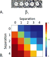
The pattern of responses in a border salience experiment along the β\ -axis. Panel A: locations of the five test points along the β\-axis, equally spaced from β\ = −0.75 to β\ = +0.75. Panel B: The frequency that a border between one pair of patches was judged more salient than the border between a second pair. White indicates a border pair that was not presented. Data are grouped according to the veridical separation in the domain, illustrated in Panel A. For a breakdown according to individual pairs of test points, see Supplementary Figure 1. Subject: KP.
Figure 8
Figure 8
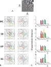
Multidimensional scaling of border salience judgments along the coordinate axes. The locations of the five test points {x2,x1,x0,x1,x2} are indicated by their color, referenced to the key in upper left; they are equally-spaced along the axes with ranges of ±0.25 (γ), ±0.45 (β_), ±0.75 (β\), ±1.0 (θ_), and ±0.85 (α). The scale bar indicates a distance (d(xi,xj)) in equation 2) of 0.1, in the absolute units of image statistics. For each plot, the positional uncertainty (σ in equation 2) required to account for the salience judgments is given the “2D” column of Table 2. Contour lines, where visible, indicate 95% confidence regions. Four subjects.
Figure 9
Figure 9
Comparison of thresholds determined from the segmentation task (abscissa) with uncertainties σ (2D fit, Table 2) determined from the border salience task. Panel A: Data from the five on-axis experiments (γ, β_, β\, θ, α). The four points for each image statistic correspond to data from the four subjects. Panel B: The corresponding analysis for data in the (β_, β|) and (β\, β/) -planes. Square symbols: same-sign coordinates; triangular symbols: opposite-sign coordinates. Solid lines in Panels A and B are linear regressions fit by least-squares. Regression parameters in Panels A and B are non-overlapping: slopes (and 95% confidence limits) are 0.64 (0.54 to 0.75) in A, 0.16 (−0.09 to 0.41) in B; intercepts are 0.02 (−0.04 to 0.07) in A, 0.25 (0.15 to 0.35) in B. Panel C: ratio of uncertainty σ to threshold, as a function of threshold. Filled symbols from panel A, open symbols from panel B.
Figure 10
Figure 10
The pattern of responses in border salience experiments in the (β\, β/) -plane. Panel A: locations of the five test points along the β\ = β/ -line (cyan) and the β\ = −β/ -line (brown). Panel B: The frequency that a border between one pair of patches was judged more salient than the border between a second pair, for test points along the β\ = β/ -line. Other details as in Figure 7B. Panel C: As in Panel B, but for test points along the β\ = −β/ -line. For a breakdown according to individual pairs of test points, see Supplementary Figure 2. Subject: KP.
Figure 11
Figure 11
Multidimensional scaling of border salience judgments in selected coordinate planes in off-axis directions: cyan for same-sign directions, brown for opposite-sign directions. Other details as in Figure 8.

Similar articles

Cited by

References

    1. Aronov D, Victor JD. Non-Euclidean properties of spike train metric spaces. Phys Rev E Stat Nonlin Soft Matter Phys. 2004;69(6 Pt 1):061905. - PMC - PubMed
    1. Baylor DA, Nunn BJ, Schnapf JL. Spectral sensitivity of cones of the monkey macaca fascicularis. J Physiol (Lond) 1987;390:145–160. - PMC - PubMed
    1. Bushdid C, Magnasco MO, Vosshall LB, Keller A. Humans can discriminate more than 1 trillion olfactory stimuli. Science. 2014;343(6177):1370–1372. doi: 10.1126/science.1249168. - DOI - PMC - PubMed
    1. Catz O, Kampf M, Nachson I, Babkoff H. From theory to implementation: building a multidimensional space for face recognition. Acta Psychol (Amst) 2009;131(2):143–152. doi: 10.1016/j.actpsy.2009.03.010. - DOI - PubMed
    1. Chubb C, Landy MS, Econopouly J. A visual mechanism tuned to black. Vision Res. 2004;44(27):3223–3232. - PubMed

Publication types