. 2017 Nov 1:234:38-45.
doi: 10.1016/j.foodchem.2017.04.098. Epub 2017 Apr 18.

The contribution of alliaceous and cruciferous vegetables to dietary sulphur intake

Affiliations

The contribution of alliaceous and cruciferous vegetables to dietary sulphur intake

Joanne F Doleman et al. Food Chem. .

Abstract

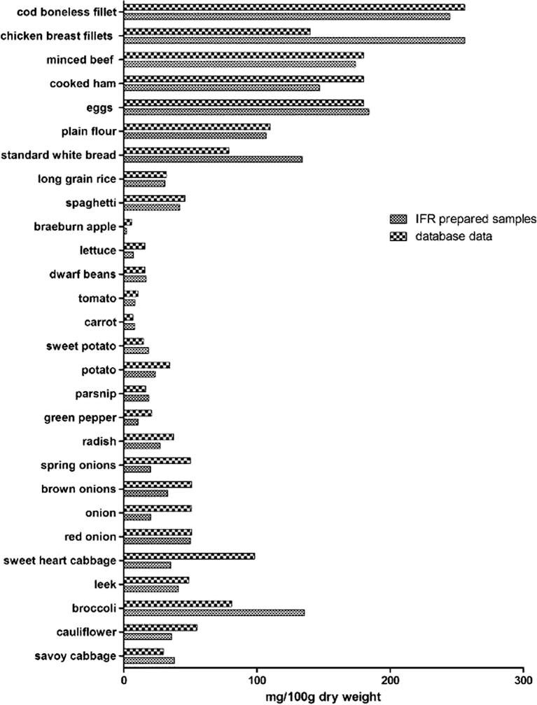
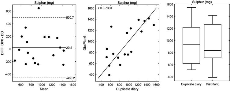
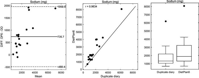
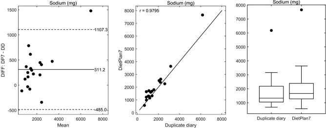
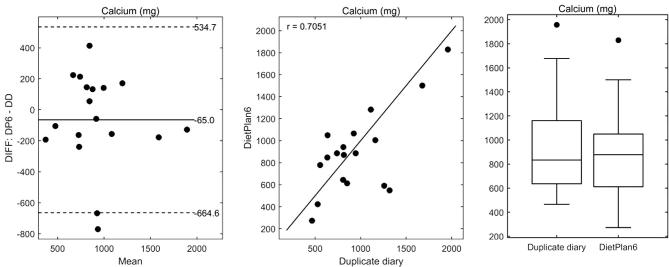
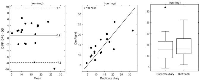
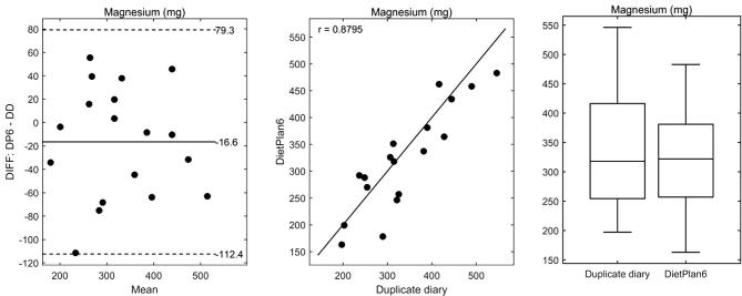
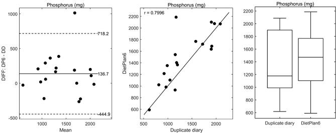
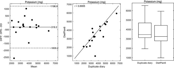
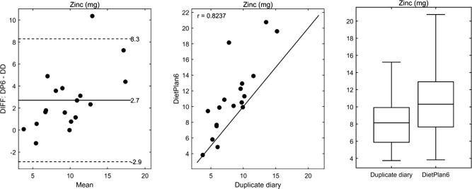
Despite its importance in many areas of human metabolism, there are no recommended daily intake guide lines for sulphur. It is generally assumed that most dietary sulphur originates from intake of methionine and cysteine. We estimated sulphur intake from food diaries, and validated the results with the use of a duplicate diet analyses. Sulphur intake estimations were highly correlated with that obtain through an elemental analysis of duplicate diets, with a mean±sd daily intakes of 956±327.9mg estimated from diet diary analyses and 935±329.9mg estimated by a duplicate diet analyses. Sulphur intake from alliaceous and cruciferous vegetables contributed up to 42% of total sulphur intake. Daily intake estimation comparisons through diet diary analyses and duplicate diet for other elements showed good agreement, except for sodium and zinc, in which analyses of 24h diet dairies overestimated intake by 35% and 52%, respectively.

Keywords: Diet diary; Duplicate diet; Sulphate; Sulphur; Sulphur amino acids (SAA).


Figures

Fig. 1
Fig. 1
Sulphur content of 28 commonly consumed foods from the sulphur database versus Eurofins UK analysis of IFR in-house prepared samples. The sulphur content in mg per 100 g fresh weight of each food tested was comparable to that in the sulphur database, although some differences are observed. There does not appear to be any obvious systematic bias in the analysis.
Fig. 2
Fig. 2
Sulphur intake estimates of 18 × 24-h dietary intake diaries using DietPlan6 and duplicate diet analysis. Left panel, Bland and Altman plot (Bland & Altman, 1986) of the differences, DietPlan6 – duplicate diary, against the mean of the two estimates. Also shown is the bias given as the mean difference and the 95% limits of agreement (mean difference ± 2 × standard deviation). Central panel, scatterplot of DietPlan6 estimates against duplicate diary values. Also shown is the Pearson correlation between the two methods and the line of unity. Right panel, boxplots summarising the distribution of the two estimates.
Fig. 3
Fig. 3
Sodium intake estimates of 18 × 24-h dietary intake diaries using DietPlan6 and duplicate diet analysis. Left panel, Bland and Altman plot (Bland & Altman, 1986) of the differences, DietPlan6 – duplicate diary, against the mean of the two estimates. Also shown is the bias given as the mean difference and the 95% limits of agreement (mean difference ± 2 × standard deviation). Central panel, scatterplot of DietPlan6 estimates against duplicate diary values. Also shown is the Pearson correlation between the two methods and the line of unity. Right panel, boxplots summarising the distribution of the two estimates.
Supplementary Figure 1
Updated Sodium: Sodium intake as estimated by updated databases in diet diary analysis data versus duplicate diet analysis. New Sodium data was obtained from the UK Department of Health updated food composition dataset (PublicHealthEngland, 2015) Left panel, Bland and Altman plot (Bland & Altman, 1986) of the differences, DietPlan7 – duplicate diary, against the mean of the two estimates. Also shown is the bias given as the mean difference and the 95% limits of agreement (mean difference ± 2 × standard deviation). Central panel, scatterplot of DietPlan7 estimates against duplicate diary values. Also shown is the Pearson correlation between the two methods and the line of unity. Right panel, boxplots summarising the distribution of the two estimates.
Supplementary Figure 2
Calcium: Calcium intake estimates of 18 × 24-hour dietary intake diaries using DietPlan6 and duplicate diet analysis. Left panel, Bland and Altman plot, (Bland & Altman, 1986) of the differences, DietPlan6 – duplicate diary, against the mean of the two estimates. Also shown is the bias given as the mean difference and the 95% limits of agreement (mean difference ± 2 × standard deviation). Central panel, scatterplot of DietPlan6 estimates against duplicate diary values. Also shown is the Pearson correlation between the two methods and the line of unity. Right panel, boxplots summarising the distribution of the two estimates.
Supplementary Figure 3
Iron: Iron intake estimates of 18 × 24-hour dietary intake diaries using DietPlan6 and duplicate diet analysis. Left panel, Bland and Altman plot (Bland & Altman, 1986) of the differences, DietPlan6 – duplicate diary, against the mean of the two estimates. Also shown is the bias given as the mean difference and the 95% limits of agreement (mean difference ± 2 × standard deviation). Central panel, scatterplot of DietPlan6 estimates against duplicate diary values. Also shown is the Pearson correlation between the two methods and the line of unity. Right panel, boxplots summarising the distribution of the two estimates.
Supplementary Figure 4
Magnesium: Magnesium intake estimates of 18 × 24-hour dietary intake diaries using DietPlan6 and duplicate diet analysis. Left panel, Bland and Altman plot (Bland & Altman, 1986) of the differences, DietPlan6 – duplicate diary, against the mean of the two estimates. Also shown is the bias given as the mean difference and the 95% limits of agreement (mean difference ± 2 × standard deviation). Central panel, scatterplot of DietPlan6 estimates against duplicate diary values. Also shown is the Pearson correlation between the two methods and the line of unity. Right panel, boxplots summarising the distribution of the two estimates.
Supplementary Figure 5
Phosphorous: Phosphorous intake estimates of 18 × 24-hour dietary intake diaries using DietPlan6 and duplicate diet analysis. Left panel, Bland and Altman plot (Bland & Altman, 1986) of the differences, DietPlan6 – duplicate diary, against the mean of the two estimates. Also shown is the bias given as the mean difference and the 95% limits of agreement (mean difference ± 2 × standard deviation). Central panel, scatterplot of DietPlan6 estimates against duplicate diary values. Also shown is the Pearson correlation between the two methods and the line of unity. Right panel, boxplots summarising the distribution of the two estimates.
Supplementary Figure 6
Potassium: Potassium intake estimates of 18 × 24-hour dietary intake diaries using DietPlan6 and duplicate diet analysis. Left panel, Bland and Altman plot (Bland & Altman, 1986) of the differences, DietPlan6 – duplicate diary, against the mean of the two estimates. Also shown is the bias given as the mean difference and the 95% limits of agreement (mean difference ± 2 × standard deviation). Central panel, scatterplot of DietPlan6 estimates against duplicate diary values. Also shown is the Pearson correlation between the two methods and the line of unity. Right panel, boxplots summarising the distribution of the two estimates.
Supplementary Figure 7
Zinc: Zinc intake estimates of 18 × 24-h dietary intake diaries using DietPlan6 and duplicate diet analysis. Left panel, Bland and Altman plot (Bland & Altman, 1986) of the differences, Dietplan6 – duplicate diary, against the mean of the two estimates. Also shown is the bias given as the mean difference and the 95% limits of agreement (mean difference ± 2 × standard deviation). Central panel, scatterplot of DietPlan6 estimates against duplicate diary values. Also shown is the Pearson correlation between the two methods and the line of unity. Right panel, boxplots summarising the distribution of the two estimates.

References

    1. Armah C.N., Derdemezis C., Traka M.H., Dainty J.R., Doleman J.F., Saha S.…Mithen R.F. Diet rich in high glucoraphanin broccoli reduces plasma LDL cholesterol: Evidence from randomised controlled trials. Molecular Nutrition and Food Research. 2015;59(5):918–926. - PMC - PubMed
    1. Ashwell M. 4: The COMA Report on Dietary Reference Values. Nutrition Bulletin. 1991;16(3):132–135.
    1. Bland J.M., Altman D.G. Statistical methods for assessing agreement between two methods of clinical measurement. Lancet. 1986;1(8476):307–310. - PubMed
    1. Block E. The Organosulfur Chemistry of the Genus Allium – Implications for the Organic-Chemistry of Sulfur. Angewandte Chemie-International Edition in English. 1992;31(9):1135–1178.
    1. Borlinghaus J., Albrecht F., Gruhlke M.C., Nwachukwu I.D., Slusarenko A.J. Allicin: Chemistry and biological properties. Molecules. 2014;19(8):12591–12618. - PMC - PubMed

LinkOut - more resources