A Model of Fast Hebbian Spike Latency Normalization

Abstract

Hebbian changes of excitatory synapses are driven by and enhance correlations between pre- and postsynaptic neuronal activations, forming a positive feedback loop that can lead to instability in simulated neural networks. Because Hebbian learning may occur on time scales of seconds to minutes, it is conjectured that some form of fast stabilization of neural firing is necessary to avoid runaway of excitation, but both the theoretical underpinning and the biological implementation for such homeostatic mechanism are to be fully investigated. Supported by analytical and computational arguments, we show that a Hebbian spike-timing-dependent metaplasticity rule, accounts for inherently-stable, quick tuning of the total input weight of a single neuron in the general scenario of asynchronous neural firing characterized by UP and DOWN states of activity.

Keywords: STDP; homeostasis; metaplasticity; oscillations; synapse memory; synchrony.

Figure 1

The model without leak (left column) vs. the model with leak (right column). (A) In both models the neurons spike when their membrane potential reaches a threshold θ_v after which it is reset to a value V_r and held at that value for τ_ref ms. In the model without leak (a), the neuron receives current-based input whereas in the model with leak (b), the input is conductance-based and the membrane potential decays exponentially. The spikes are shown as stars. We refer to the purple spikes as “distinguished” spikes (DSPs). They block other postsynaptic spikes from receiving that label for a period of T_burst ms. (B) Network models. A single target neuron that receives input from a population (a). In the model with leak (b), the neuron additionally receives constant noise input with weight w_n at rate ν. The synapses are binary and can be either weak (light gray), with weight w_w, or strong, with weight w_s (dark gray). (C) Input spike model. (a) Each input neuron spikes once at a time chosen uniformly at random within a short interval. Presynaptic spikes which occur before (after) the postsynaptic spike lead to a potentiation (depression) signal which is highlighted with a green (red) shaded region. (b) The input spikes are modeled as an inhomogeneous Poisson process. The input neurons switch between a high rate UP phase and a low rate DOWN phase (orange curve with respect to right y-axis). The presynaptic spikes which occur in a window before (after) the distinguished postsynaptic spike trigger potentiation (depression) signals and the window is highlighted in green (red). (D) Learning rule. Each synapse has a memory trace m(t) that is modified for certain spike pair events, similar to standard STDP. (a) Potentiation and depression signals are always with respect to spike pairs and we track the spikes with the variables 𝟙_pre and 𝟙_post. The memory in the model without leak contains the last M potentiation and depression signals and the memory trace is the fraction of potentiation signals. (b) Variables to define distinguished spikes (DSPs), potentiation and depression signals, and the memory trace m(t) (see Section 2.3 for details).

Figure 2

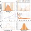
Principles of the intrinsic homeostasis mechanism in the model without leak. Orange curves correspond to a setting with “deterministic” synapses, which reliably transmit spikes, and the purple curves correspond to a setting with “probabilistic” synapses that transmit spikes with probability p_r = 0.5. (A) Probability of a potentiation signal conditioned on the postsynaptic neuron spiking and the synapse being reliable. The gray area corresponds to the value of the memory trace where synapses neither potentiate nor depress. (B) Expected drift toward the stable input weight in each weight update as a function of the total input weight. The arrows correspond to the stable input weights to which the input weight converges in the two settings (the stable state). (C) Convergence to the stable input weight for three different starting conditions in each setting, where one is the stable state. The curves represent the mean over 50 trials and the envelope corresponds to a standard deviation estimate. (D) The total input weight, which is the same as the number of strong synapses d_s, distribution for deterministic synapses after applying 200 weight updates (darker orange) when d_s = 30 before the first weight update. The total input weight distribution is similar to a setting where potentiation is forbidden (p_w→s = 0, lighter orange), which illustrates that the negative feedback does not undershoot the stable state by much. For all panels, M, θ_D and θ_P, p_w→s, and p_s→w are set as in Table 1.

Figure 3

Noisy input and the random order assumption in the model without leak (Section 3.1.2). (A) The stable state $d_s^{*}$ scales by 1/p_r for probabilistic synapses. The initial value of d_s is set to 20/p_r for each p_r and the plot shows the mean value of d_s · p_r after 50 weight updates over 100 trials. (B–C) From a fixed order to a random order. Spike order distributions that are not uniform are considered in these panels. The parameter σ brings them from a fixed order (σ = 0) to a uniform order (σ → ∞). (details are explained in Section 3.1.2). Initially, each synapse is strong independently, with probability 4θ_v/d. (B) Small variability brings the stable state $d_s^{*}$ close to same state as when the spike order is uniform. (C) The plasticity mechanism prefers early neurons when σ is small. This is reflected by the mean index of the strong synapses, which are indexed from 1 to d in ascending order of expected spike time. However, as σ increases, the early neurons become less distinguishable from later neurons. In (B,C) each data point is the mean of 250 trials, where for each trial 250 weight updates are simulated. For all panels, the plasticity parameters are chosen as in Table 1 and the envelopes represent standard deviation estimates.

Figure 4

Plasticity vs. stability in the model with leak (Section 3.2.1). (A) Distribution of the memory trace in a static setting, with p_s→w = p_w→s = 0 and d_s = 20 strong input synapses. The colored vertical bars represent the target interval [θ_D, θ_P] used in (B,C). (B) The mean fraction of synapses whose memory trace lies outside the interval [θ_D, θ_P] in a static setting. (C) The trade-off between the number of weight changes in the stable state and convergence time to the stable state. The light purple curve shows the mean number of weight changes per UP phase over all input synapses. The dark purple curve shows the mean time for the weights to converge from d_s = 80 to d_s = 25. The ticks on the x-axis are colored and correspond to the thresholds in (A) and curves in (B). In this setup, the number of strong synapses in the stable state is d_s = 20. This is achieved by choosing p_s→w and p_w→s such that they satisfy the equation d_sp_s→w = (d − d_s)p_w→s; i.e., p_w→s = 0.0625 and p_s→w = 0.25. The error bars represent standard deviation estimates. (D) Comparison of the effect p_s→w and p_w→s have on convergence. In this figure, θ_D = −5.1 and θ_P = −1.1, and three different values of p_w→s (0.05, 0.25, and 1.0) are compared (the corresponding p_s→w values are 0.01, 0.06, and 0.25). If too many synapses change their weight simultaneously because of a small target interval and large weight change probabilities, then the weights can overshoot the stable state and oscillate around it. (E,F) Stability for different weight distributions. (E) Density function for two different weight distributions of the strong synapses. The dark orange is the density function of $\mathcal{N}(40,5)$, and the light orange is the density function for the random experiment, where we either draw the weight from the distribution $\mathcal{N}(35,5)$ or $\mathcal{N}(45,5)$ based on a fair coin toss. (F) The corresponding memory trace distribution for each weight distribution when d_s = 24 in a static setting with p_s→w = p_w→s = 0. By choosing θ_D = −16 and θ_P = 5, the weight remains unchanged for both weight distributions over a period of 50 s and oscillating input (data not shown). In (A) the distribution is obtained by sampling memory traces of all d synapses after a simulation of 500 UP phases in 250 trials. In (B) each data point is the mean of 100 trials. In (C) each curve is the average over 40 trials. In (D) each curve is the average over 200 trials with a data point every 125 ms. For all panels, error bars and envelopes represent standard deviation estimates. In (F) the distribution is sampled from 100 synapses over 200 trials of a 50 second simulation.

Figure 5

Comparison of short and long UP phases. (A,B) Dependence of number of strong input synapses d_s and relative spike time on the lengths of UP phases. We set T_D = 1000.0 ms and we set T_burst = 1000.0 such that there can be only one DSP per UP phase. (A) shows that for long UP phases the mechanism normalizes d_s. (B) shows that for short UP phases the mechanism normalizes the relative spike time r within an UP phase. (C) Depression is stronger for sufficiently long UP phases. For two different rate functions the postsynaptic spikes are drawn on top of an UP phase where darker spikes represent DSPs. The black bar represents the learning windows. The time window of the depression signal is completely within the UP phase if the UP phase is long. This increases the expected number of depression signals. To compensate, the input weight needs to decrease in order to correct the ratio of potentiation to depression signals. (D) Weight change for short UP phases of 30 ms with d_s = 17 at t = 0 (left panel) and long UP phases of 0.5 s with d_s = 27 at t = 0 (right panel). We show 20 example runs with one highlighted in orange for clarity.

Figure 6

Heterogeneous and multimodal weights in the model without leak (Section 3.2.3). (A,B) Heterogeneous weights. (A) Input convergence with the spike threshold θ_v adapted to the synaptic weights. (B) Comparison between the distribution of strong synaptic weights (lognormal distribution, shaded) and the strong weights after convergence (dots). (C,D) Multimodal synapses. Two different weight update rules are presented: one additive and one multiplicative (see Section 2.5 for details). (C) Convergence for the two different setups where all the synapses start with weight 10 and θ_v is set to 100. (D) The input weight distributions are compared for the multimodal weight update rules in (C) after 250 extra weight updates. The additive weight update rule produces a bimodal weight distribution whereas the multiplicative one produces a unimodal distribution. None of the update rules imposes a hard upper bound on the weights and all resulting weights are less than 10, which was the starting weight of the synapses. For all panels, the parameters were chosen as in Table 1 unless otherwise specified. In (A,C) each curve is the mean of 30 and, respectively, 100 trials; the envelopes represent a standard deviation estimate. In (B) the distribution is obtained from 5.000 trials, where in each one 50 weight updates were simulated.

Figure 7

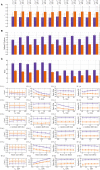
Robustness against varying input parameters in the model with leak (Section 3.2.4). (A–C) Results for two different sets of plasticity parameters corresponding to r = 1/3 (purple) and r = 1/2 (orange) in Table 3 are shown. Three parameters of the input are varied: the length of an UP phase T_U; the number of input neurons d; and the length of a DOWN phase T_D. (A) r, the expected time of the first postsynaptic spike within an UP phase scaled by the UP phase length. The plasticity parameters fix r; thus, varying the input parameters has a negligible effect on it. (B) Variations in the number of spikes per UP phase. The number of spikes per UP phase depends on r, but it also has a mild dependence on the refractory period and the reset potential, which explains the variations seen when varying T_U. (C) Output rate variations. The rule does not fix the output rate of a neuron: the rate depends mainly on T_U and T_D. (D) Single parameter variations. Variations for six different parameters are shown. The darker colored curves correspond to the same plasticity parameters as in the top three panels, and the lighter colored curves correspond to a setup with no positive feedback (p_w→s = 0). The first row is for T_U, the second is for T_D, the third is for random phase shifts of the input neurons, the fourth is for d, the fifth is for the noise rate ν, and the sixth is for the membrane capacitance (for details see Section 3.2.4). The orange curves start with d_s = 17 and the purple curves start with d_s = 25. Each data point in (A–C) is the mean of 40 trials and in (D) the mean of 10 trials. The error bars represent standard deviation estimates. For each trial, the process was simulated for 200 UP phases to reach the stable state and then the data points were collected over a continued simulation of 200 UP phases (r, rate, spikes per UP phase), or at the end (d_s).

Figure 8

(A) Advantage of DSPs (Section 3.2.5). With DSPs in the model with leak, the variance of the memory trace is considerably smaller than for an all-to-all rule. The curves show the mean memory trace value when varying the number of strong inputs d_s in a static setting with p_s→w = p_w→s = 0. The orange curve corresponds to the SLN rule. The purple curve corresponds to a rule where all pre–post and post–pre spike pairs within an UP phase trigger learning signals. (B) Constant rate input at 40 Hz in the model with leak (Section 3.2.6). The two different sets of plasticity parameters from Table 3 are compared. For each setting, the number of strong synapses d_s is initially set in the stable state for the oscillating input. For the r = 1/3 parameters, all the synapses increase their weights since the synapses receive potentiation signals half of the time instead of one-third of the time, which they expect. For the r = 1/2 parameters, there is no such disagreement and for the r = 2/3 parameters it is the opposite and the input weight decreases to a point where activation becomes unreliable. In (A) the mean is taken after a 50-s-simulation over 10 trials, where in each trial samples are taken from all 100 synapses. In (B) the curves show means of 50 trials. In both panels the envelopes represent standard deviation estimates.

References

1. Abbott L. F., Nelson S. B. (2000). Synaptic plasticity: taming the beast. Nat. Neurosci. 3, 1178–1183. 10.1038/81453 - DOI - PubMed
1. Abraham W. C. (2008). Metaplasticity: tuning synapses and networks for plasticity. Nat. Rev. Neurosci. 9, 387–387. 10.1038/nrn2356 - DOI - PubMed
1. Abraham W. C., Bear M. F. (1996). Metaplasticity: the plasticity of synaptic plasticity. Trends Neurosci. 19, 126–130. 10.1016/S0166-2236(96)80018-X - DOI - PubMed
1. Babadi B., Abbott L. F. (2010). Intrinsic stability of temporally shifted spike-timing dependent plasticity. PLoS Comput. Biol. 6:e1000961. 10.1371/journal.pcbi.1000961 - DOI - PMC - PubMed
1. Bair W., Koch C. (1996). Temporal precision of spike trains in extrastriate cortex of the behaving Macaque monkey. Neural Comput. 8, 1185–1202. 10.1162/neco.1996.8.6.1185 - DOI - PubMed
LinkOut - more resources